Week 5 - Rayleigh Taylor Instability
Rayleigh Taylor Instability
<!-- [if !supportLists]-->1. <!--[endif]-->What are some practical CFD models that have been based on the mathematical analysis of Rayleigh Taylor waves? In your own words, explain how these mathematical models have been adapted for CFD calculations.
<!-- [if !supportLists]-->2. <!--[endif]-->Perform the Rayleigh Taylor instability simulation for 2 different mesh sizes with the base mesh being 0.5 mm. Compare the results by showing the animations( Attach them from your google drive). Observe the differences in the animation and explain the effect of mesh size on simulation. Also, explain why a steady-state approach might not be suitable for these types of simulation.[ Choose Air and Water for this simulation]
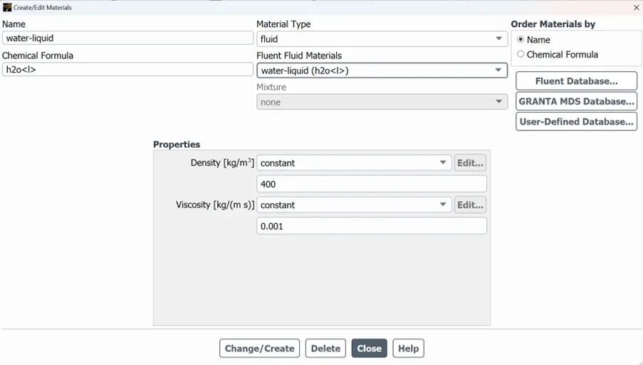
<!-- [if !supportLists]-->3. <!--[endif]-->Run one more simulation with water and user-defined material(density = 400 kg/m3, viscosity = 0.001 kg/m-s) for refined mesh.
<!-- [if !supportLists]-->4. <!--[endif]-->Define the Atwood Number. Find out the Atwood number for both the cases and explain how the variation in Atwood number in the above two cases affects the behavior of the instability.
INTRODUCTION
<!-- [if !supportLists]-->· <!--[endif]-->Rayleigh – Taylor instability is a fundamental fluid dynamics phenomenon that occurs when a denser fluid overlies a lighter one in a gravitational field. It leads to the formation of intricate, mushroom-like structures aas the heavier fluid penetrates into the lighter one. Understanding and simulating Rayleigh – Taylor instability is crucial in various scientific and engineering applications, such as astrophysics, nuclear fusion and mixing in chemeical processes.
Mathematical Models for CFD:
<!-- [if !supportLists]-->· <!--[endif]-->To simulate Rayleigh – Taylor instability, CFD models adopt mathematically equations, particularly the Navier – Stokes equations and the contuinity equation. These models are discretized over a computational mesh to describe mesh to describe of fluid behavior.
Effects of Mesh Size and Need for Transient Simulations:
<!-- [if !supportLists]-->· <!--[endif]-->Mesh size significantly impacts simulation accuracy, with the smaller meshes providing finer detail. For Rayleigh – Taylor instability, transient simulations are essential because this phenomenon involves evolving dynamics, making steady – state approaches unsuitable.
Atwood Number and its Impact:
<!-- [if !supportLists]-->· <!--[endif]-->The Atwood number (A) quantifies density differences between the fluids involved. A higher A signifies more substantial density differences, resulting in faster and more pronounced instability growth. Lower A values to slower mixing and less conspicuous instability features. Variations in A affect the instability’s behavoir, making it a critical parameter to consider in simulations.
1. <!--[endif]-->What are some practical CFD models that have been based on the mathematical analysis of Rayleigh Taylor waves? In your own words, explain how these mathematical models have been adapted for CFD calculations.
The Rayleigh-Taylor instability is well-studied phenomenon in fluid dynamics, and it has implications in various fields such as astrophysics, engineering, and nuclear fusion. Computational Fluid Dynamics(CFD) models based on mathematical analysis of Rayleigh-Taylor waves have been developed to simulate and understand this instability. These models typically involve solving the Navier - Stokes equations with additional physics or sub-models to capture the effects of the Rayleigh-Taylor instability. Here are some practical CFD models and techiniques based on the mathematical analysis of Rayleigh-Taylor waves.
<!-- [if !supportLists]--> 1. <!--[endif]-->Incompressible Navier-Stokes Equations:
<!-- [if !supportLists]-->· <!--[endif]-->One common approach is to solve the incompressible Navier-Stokes equations along with the contuinity equations using a numerical method such as finite difference, finite volume, or finite element methods.
<!-- [if !supportLists]-->· <!--[endif]-->The Rayleigh_Taylor interface is tracked using a level-set or volume-fluid (VOF) method, which represents the fluid interface as scalar field.
<!-- [if !supportLists]-->· <!--[endif]-->The interfacial dynamics are modelled using interfacial tracking algorithms that account for the properties on either side of the interface.
<!-- [if !supportLists]--> 2. <!--[endif]--> Reynolds-Averaged Navier-Stokes (RANS) Models:
<!-- [if !supportLists]--> RANS models, such as the k-epsilon turbulence model or the Reynolds Stress Model (RSM), can be coupled with the incompressible Navier-Stokes equations to simulate turbulent Rayleigh-Taylor flows.
<!-- [if !supportLists]-->· <!--[endif]-->These models incorporate turbulence closure schemes to account for the turbulent mixing and entertainment at the interface.
<!-- [if !supportLists]--> 3. <!--[endif]-->Large Eddy Simulation (LES):
<!-- [if !supportLists]-->· LES is a techinique used to resolve large-scale turbulent structures while modelling the smaller sclaes.
<!-- [if !supportLists]-->· <!--[endif]-->LES has been applied to Rayleigh-Taylor simulations to capture the turbulent mixing and interface dynamics with higher fidelity compared to RANS models.
<!-- [if !supportLists]--> 4. <!--[endif]-->Direct Numerical Simulations (DNS):
<!-- [if !supportLists]-->· <!--[endif]-->LES is a techinique used to resolve large-scale turbulent structures while modelling the smaller scales.
<!-- [if !supportLists]-->· <!--[endif]-->LES has been applied to Rayleigh-Taylor simulations to capture the turbulent structures and interfaces evolution.
5. Multi-Fluid Models:
<!-- [if !supportLists]-->· <!--[endif]-->Multi-fluids models explicity simulate multiple fluids with their respective properties.
<!-- [if !supportLists]-->· These models are particularly suited for situations where there are multiple immisible fluids with varying densities.
<!-- [if !supportLists]-->· They track the interfaces between fluids and model interfacial instabilities like Rayleigh-Taylor in a detailed manner.
6. Non-ideal Effects and Complex Physics:
<!-- [if !supportLists]-->· <!--[endif]-->In some practical scenerios, additional physics such as compressibility, heat transfer, or magnetic fields may be important.
Adapting mathematically models for Rayleigh-Taylor waves to CFD calculations involves discretizing the governing equations in space and time implementing numerical techniques for solving these equations on a computational grid. The key steps in adapting these models include
<!-- [if !supportLists]-->· <!--[endif]-->Setting up the initial conditions that define the fluid properties and the perturbations at the interface.
<!-- [if !supportLists]-->· <!--[endif]-->Selecting appropriate numerical schemes and methods for solving the governing equations.
<!-- [if !supportLists]-->· <!--[endif]-->Implementing boundary conditions that reflects the physical system being modeled.
<!-- [if !supportLists]-->· <!--[endif]-->Specifying the computational grid and time-stepping scheme.
<!-- [if !supportLists]-->· <!--[endif]-->Post-processing and analyzing the simulation results to understand the evolution of the Rayleigh-Taylor instability, including the growth rate, mixing, and other relevant parameters.
2. Perform the Rayleigh Taylor instability simulation for 2 different mesh sizes with the base mesh being 0.5 mm. Compare the results by showing the animations( Attach them from your google drive). Observe the differences in the animation and explain the effect of mesh size on simulation. Also, explain why a steady-state approach might not be suitable for these types of simulation.[ Choose Air and Water for this simulation]
Observe the differences in the animations from simulations with different mesh sizes and understanding why steady-state approach is unsuitable for Rayleigh-Taylor instability simulations is crucial:
Effects of mesh Size:
1. Larger Mesh (0.5mm cell size)
<!-- [if !supportLists]-->· <!--[endif]-->Coarser representation of the domain.
<!-- [if !supportLists]-->· <!--[endif]-->Less resolution in capturing small-scale features.
<!-- [if !supportLists]-->· <!--[endif]-->May underestimate mixing and result in smoother, less detailed instability development.
<!-- [if !supportLists]-->· <!--[endif]-->Smoother interface evolution and larger numerical diffusion .
2. Smaller Mesh ( 0.3 mm Cell Size)
<!-- [if !supportLists]-->· <!--[endif]-->Finer representation of the domain.
<!-- [if !supportLists]-->· <!--[endif]-->Higher resolution capturing small-scale features and intricate instability patterns.
<!-- [if !supportLists]-->· <!--[endif]-->More accurate prediction of mixing at the interface.
<!-- [if !supportLists]-->· <!--[endif]-->Capturing finer details of the instability, including smaller vortices and structures.
Why Steady-State Approach is Unsuitable:
Rayleigh-Taylor instability is a highly dynamic and time-dependent phenomenon. A steady-State approach, which assumes a stable equilibrium, is not suitable for the following reasons:
1. Continous Evolution:
<!-- [if !supportLists]-->· <!--[endif]-->Rayleigh-Taylor instability involves the continuous groth and interaction of fluids instabilities, which do not reach a steady state. The interface between the fluids is constantly changing.
2. Transient Nature:
<!-- [if !supportLists]-->· <!--[endif]-->Instabilities and mixing occur overtime, and a steady-state approach would miss crucial information about the instability’s dynaimics.\
3. Innaccurate Results:
<!-- [if !supportLists]-->· <!--[endif]-->Applying a steady-state assumptions can lead to inaccurate results and failure to capture the true behavior of the Rayleigh-Taylor instability.
CASE 1
1. Geomentry:
<!-- [if !supportLists]-->· <!--[endif]-->Open Spaceclaim.
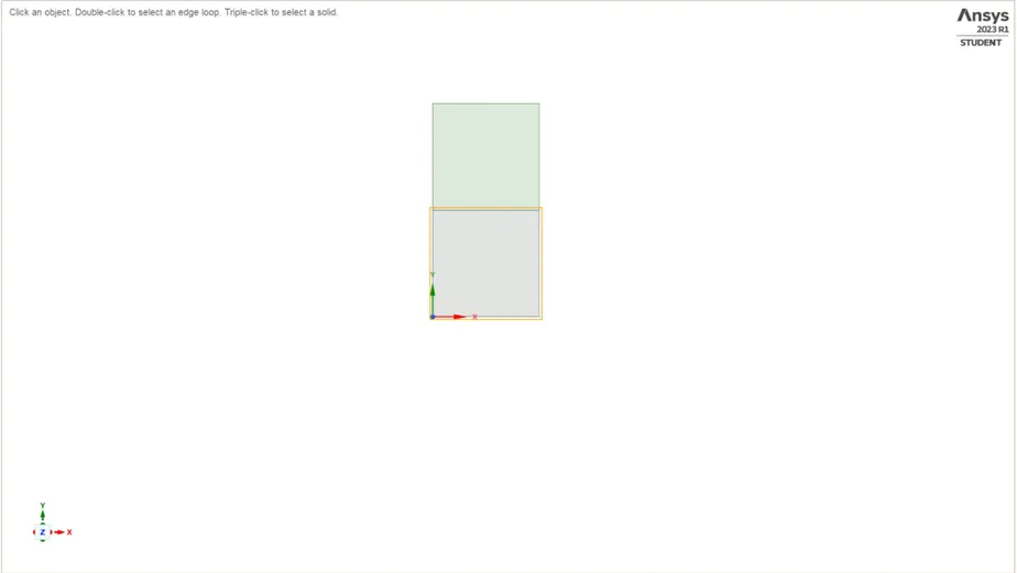
<!-- [if !supportLists]-->· <!--[endif]-->Use a Rectangle tool to create a rectangle from the orgin 20mmX20mm.
<!-- [if !supportLists]-->· <!--[endif]-->Use the Sketching tool to select the body.
<!-- [if !supportLists]-->· <!--[endif]-->Then use the pull tool command to convert a surface.
<!-- [if !supportLists]-->· <!--[endif]-->Now create a new component again by using the rectangle tool from the orgin 20X20.
<!-- [if !supportLists]-->· <!--[endif]-->Then again use the pull tool command to create a surface.
<!-- [if !supportLists]-->· <!--[endif]-->Now there are two surfaces have been created in the SpaceClaim.
<!--[endif]-->
Shareto opology :
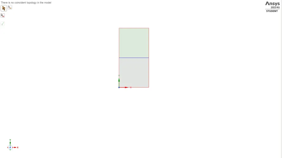
<!-- [if !supportLists]-->· <!--[endif]-->After creating the surfaces, the shareto opology is used to find the edges.
<!--[endif]-->
<!-- [if !supportLists]-->· <!--[endif]-->Enabling Shareto opology,
<!-- [if !supportLists]-->· <!--[endif]-->By clicking it, it will identify the edges between them.
<!-- [if !supportLists]-->· <!--[endif]-->After the Shareto opology the surfaces are been checked and can be interconnect to the surfaces.
<!-- [if !supportLists]-->· <!--[endif]-->After enabling the two surfaces of shareto opology, naming the sections of the surfaces in the object.
<!-- [if !supportLists]-->· <!--[endif]-->1. Sections contains Water
<!-- [if !supportLists]-->· <!--[endif]-->2. Sections contains Air
2. Meshing:
For meshing we open Meshing, where we mesh our model so that we can use it to solve our model.
Case 1Baseline Mesh
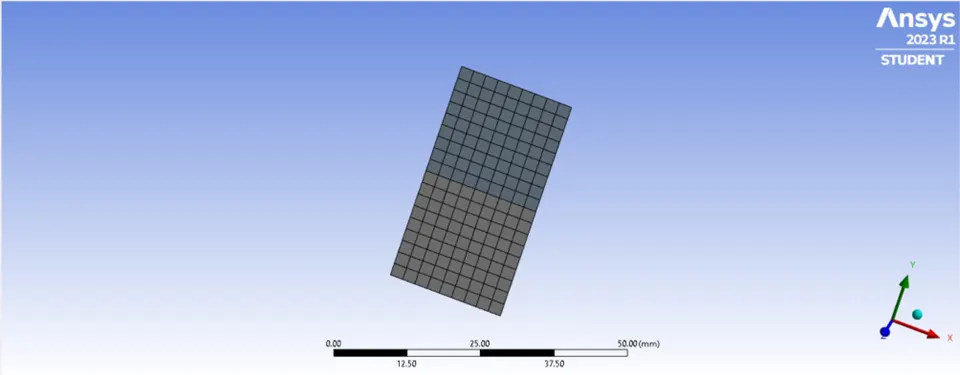
<!-- [if !supportLists]-->· <!--[endif]-->Base Mesh Size – 0.5mm
<!-- [if !supportLists]-->· <!--[endif]-->Number of elements – 3200
<!--[endif]-->
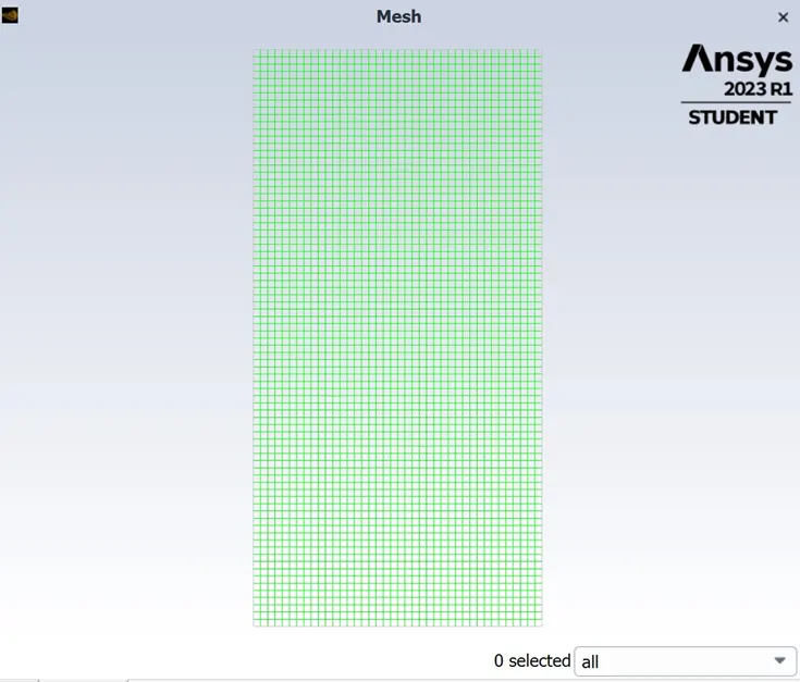
<!-- [if !supportLists]-->· <!--[endif]-->The mesh has been uploaded in the set-up.
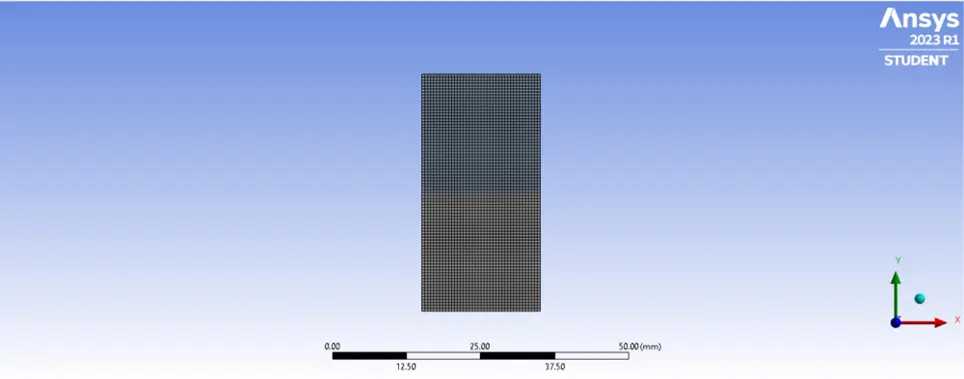
<!--[endif]-->
<!-- [if !supportLists]-->· <!--[endif]-->The baseline mesh of 0.5mm has been updated.
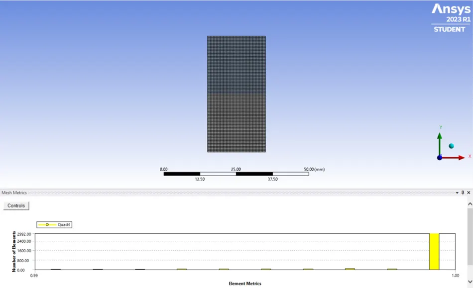
<!--[endif]-->
<!-- [if !supportLists]-->· <!--[endif]-->This plot show s the quality of the Baseline Mesh.
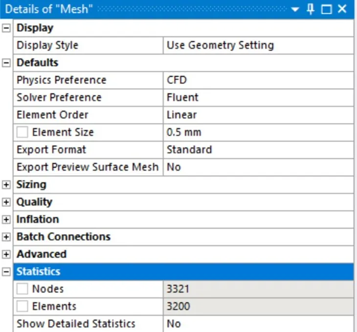
<!--[endif]-->
Named Selections:
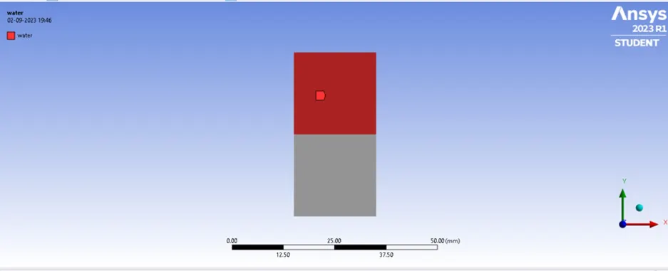
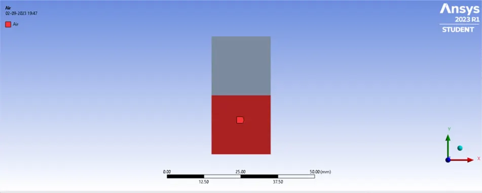
<!-- [if !supportLists]-->· <!--[endif]--> Naming the surfaces helps identify the mesh.
Water:
<!--[endif]-->
<!-- [if !supportLists]-->· <!--[endif]--> This plot represents the water.
Air:
<!--[endif]-->
<!-- [if !supportLists]-->· <!--[endif]-->This plot represents the Air.
3. Set-up:
The mesh have been updated in the set-up.
<!--[endif]-->
1. General:
<!-- [if !supportLists]-->o <!--[endif]-->Time - Transient Enabled
<!-- [if !supportLists]-->o <!--[endif]-->Gravity - It is enabled
<!-- [if !supportLists]-->o <!--[endif]-->Gravity Acceleration the Y-axis – 9.81 [m/s^2]
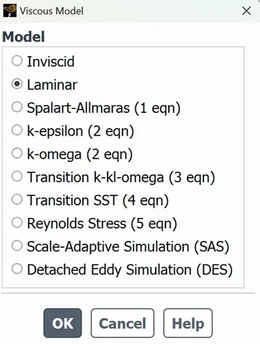
2. Viscous Model:
<!--[endif]-->
3. Material Properties
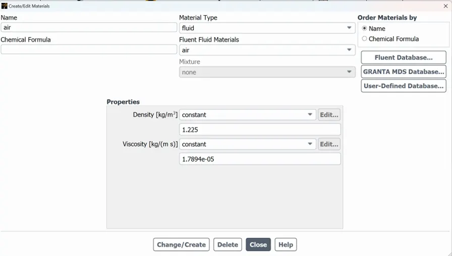
Air
<!--[endif]-->
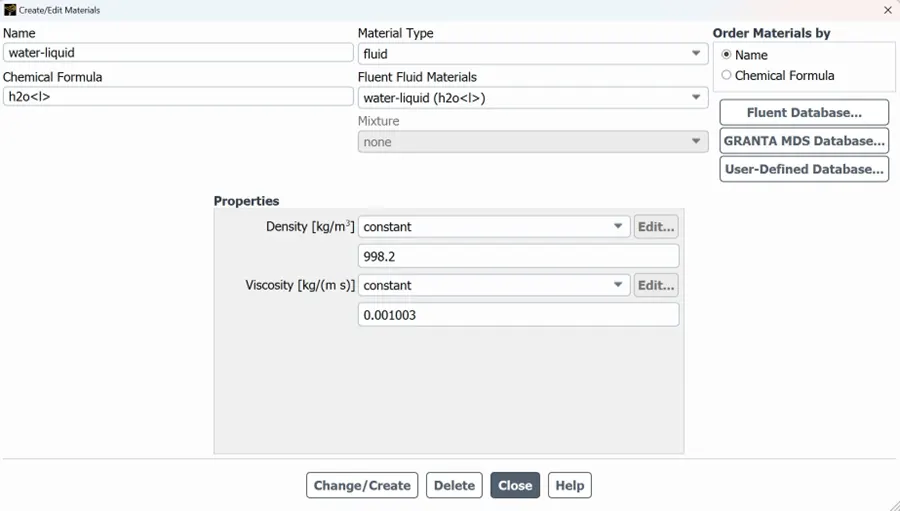
Water
<!--[endif]-->
<!-- [if !supportLists]-->· <!--[endif]-->Open the Materials manager select the default material as Air,
<!-- [if !supportLists]-->· <!--[endif]-->After clicking on Fluent Database. Select the water and add in the materials.
<!-- [if !supportLists]-->· <!--[endif]-->Now we have both Air and Water.
<!-- [if !supportLists]-->· <!--[endif]-->Change the model of Volume of Fluid in the Multi phase Model.
4. Multi-phase Model
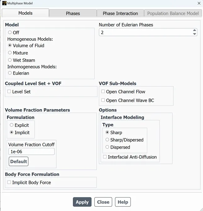
<!--[endif]-->
Phases Phase Setup
Air - Primary Phase – Air
Water - Secondary Phase – Water
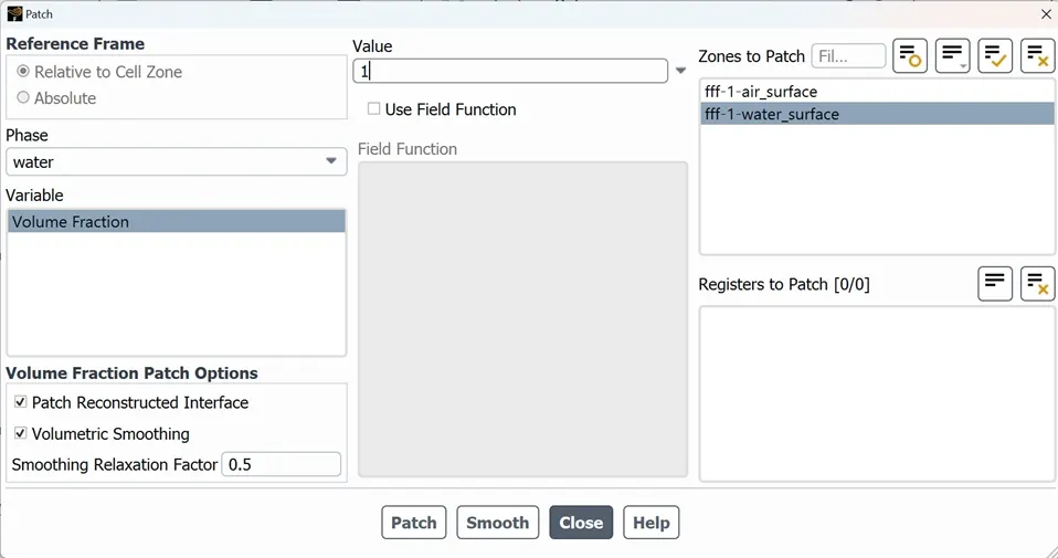
5. Patch
<!--[endif]-->
<!-- [if !supportLists]-->· <!--[endif]-->Intialization has to be done before patching the surfaces.
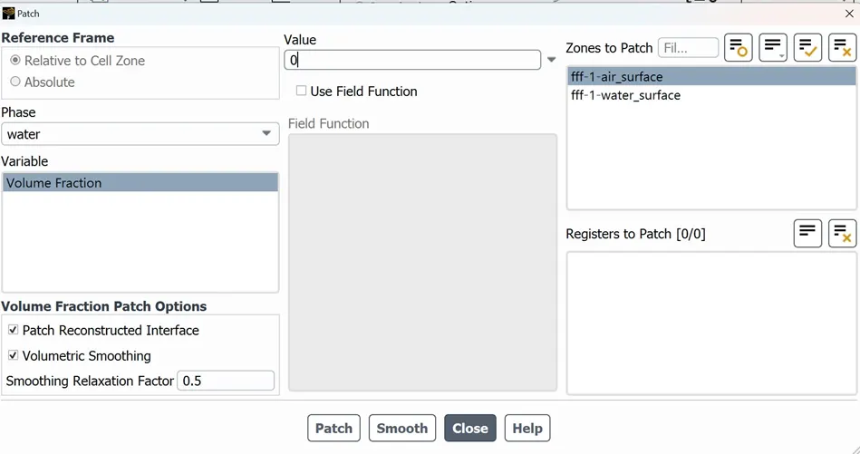
<!-- [if !supportLists]-->· <!--[endif]-->Phase
<!-- [if !supportLists]-->o <!--[endif]-->Water
<!-- [if !supportLists]-->· <!--[endif]-->Variable
<!-- [if !supportLists]-->o <!--[endif]-->Volume Fraction
<!-- [if !supportLists]-->· <!--[endif]-->Zones to patch Value
<!-- [if !supportLists]-->o <!--[endif]-->Air surface - 0
<!-- [if !supportLists]-->o <!--[endif]-->Water surface - 1
<!--[endif]-->
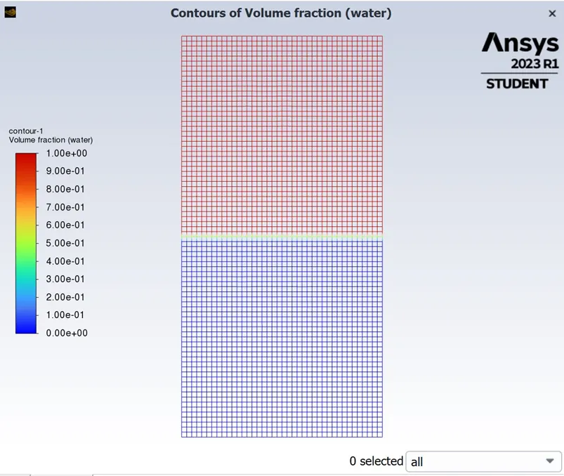
<!-- [if !supportLists]-->· <!--[endif]-->This plot shows the patched surfaces between Air and Water.
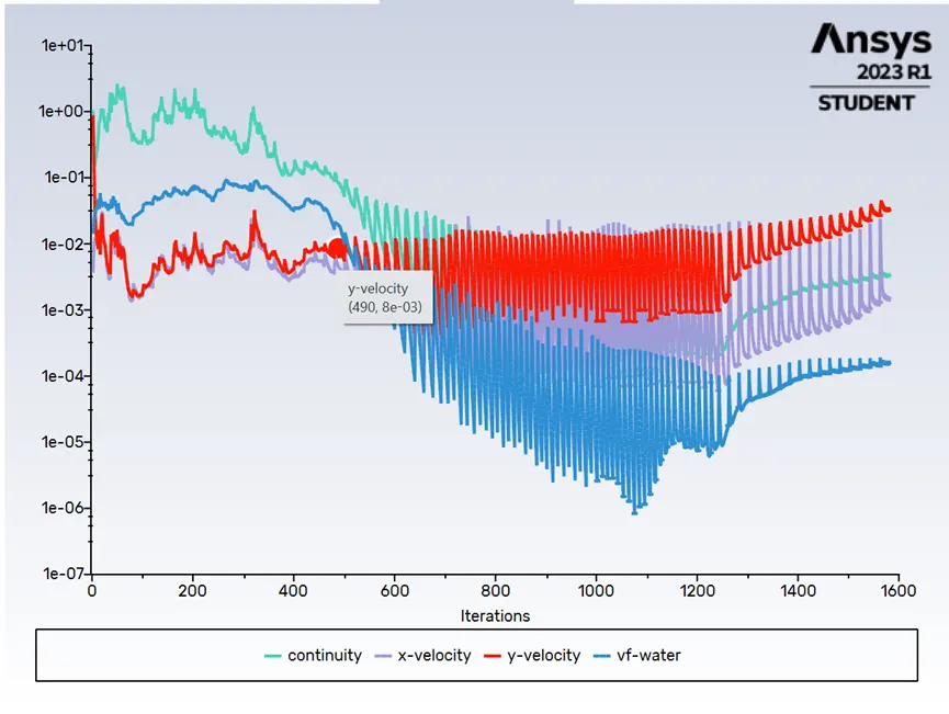
Residuals:
Time steps size [s] – 0.05
Number of Time Steps - 100
<!--[endif]-->
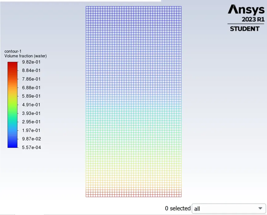
Volume of Fractions: (Water)
<!--[endif]-->
Solution Animation:
https://drive.google.com/file/d/12kJHn2qHj0HGr2UQA9EqFfic8ChUXJ6x/view?usp=sharing
<!--[endif]-->
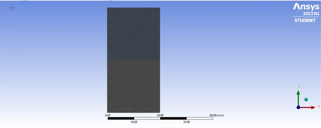
CASE 2 Refined Mesh - 1
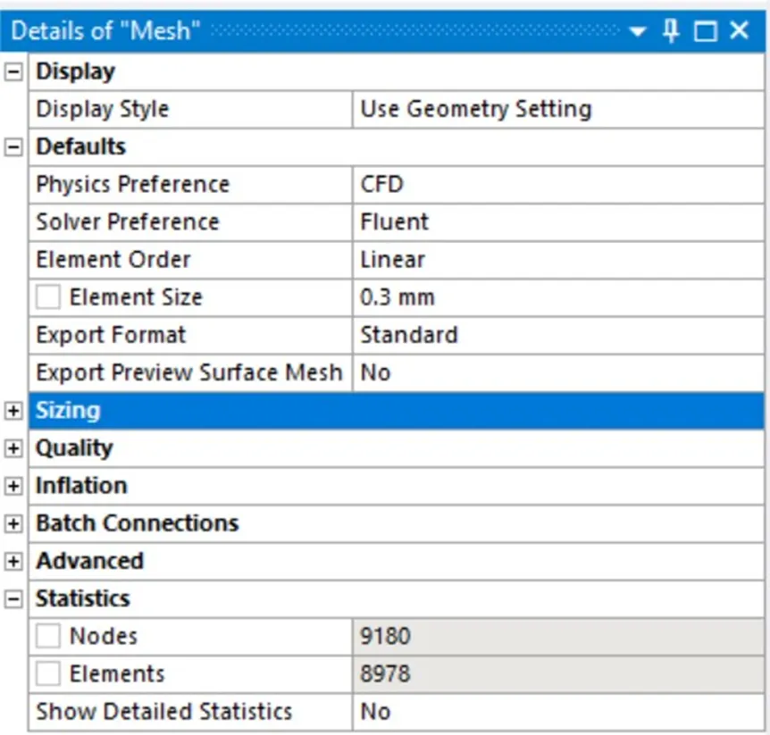
<!-- [if !supportLists]-->· <!--[endif]-->Base Mesh Size – 0.3mm
<!-- [if !supportLists]-->· <!--[endif]-->Number of elements – 8978
Mesh
<!--[endif]-->
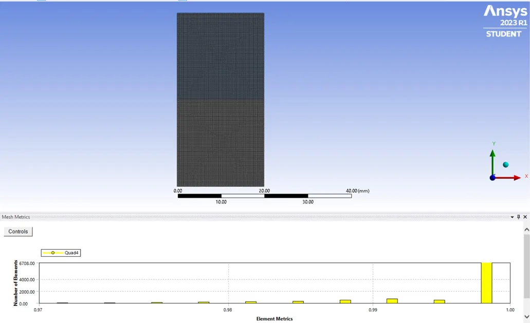
<!-- [if !supportLists]-->· <!--[endif]-->The baseline mesh of 0.3mm has been updated.
<!--[endif]-->
<!-- [if !supportLists]-->· <!--[endif]-->This plot show s the quality of the Refined Mesh.
<!--[endif]-->
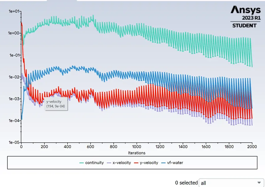
Residuals:
Time steps size [s] – 0.01
Number of Time Steps - 100
<!--[endif]-->
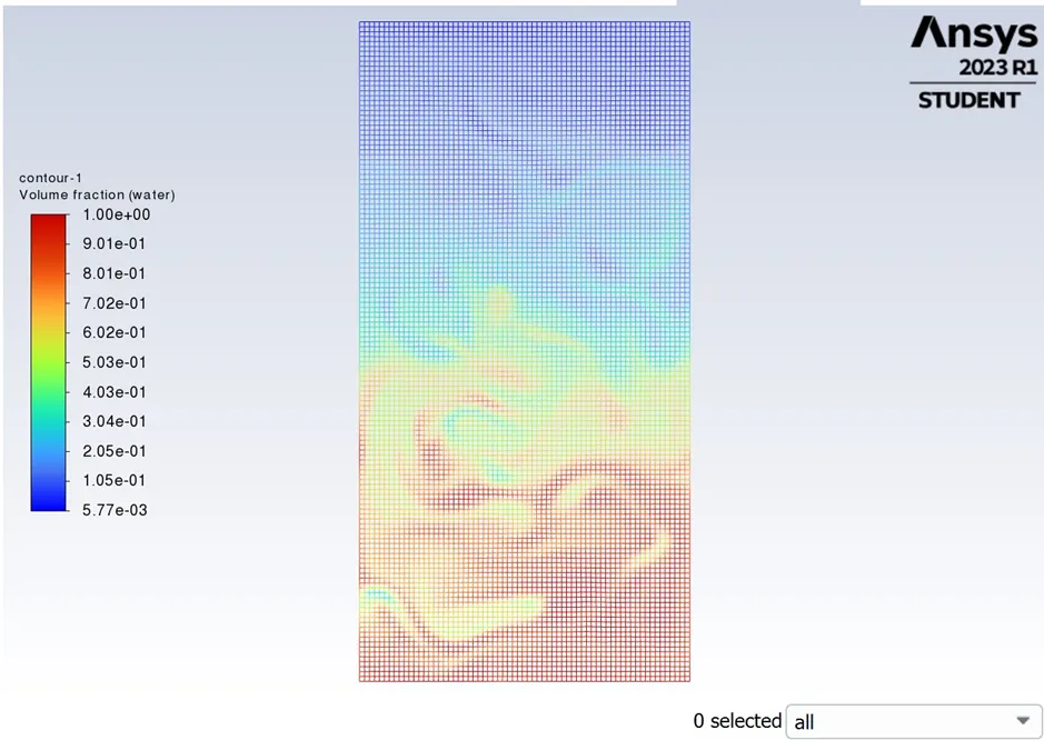
Volume of Fractions: (Water)
<!--[endif]-->
Solution Animation:
https://drive.google.com/file/d/1KW5DRP5Qg4oIF8xZ51WRYeab5UjZ5myA/view?usp=sharing
<!--[endif]-->
CASE 2 Refined Mesh - 2
<!-- [if !supportLists]-->· <!--[endif]-->Base Mesh Size – 0.4mm
<!-- [if !supportLists]-->· <!--[endif]-->Number of elements – 5000
Mesh
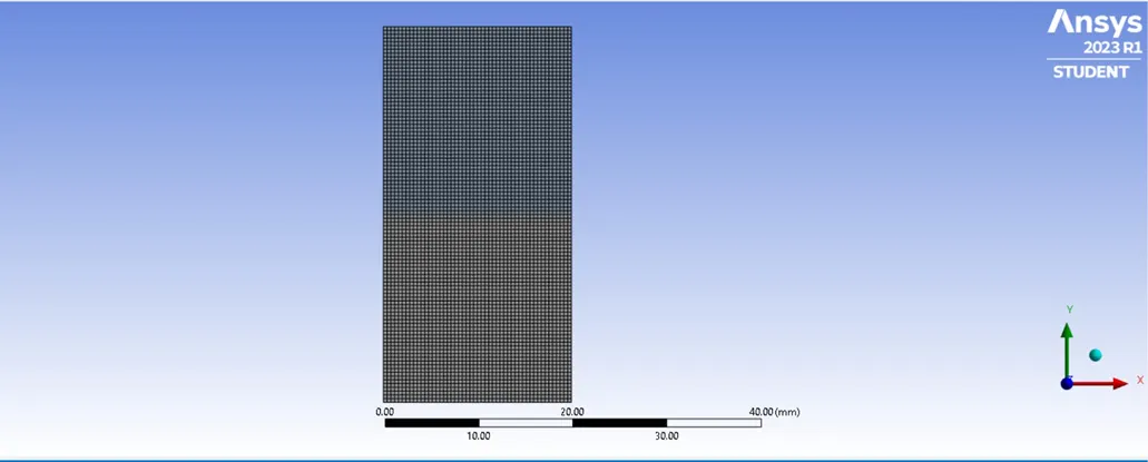
<!-- [if !supportLists]-->· <!--[endif]-->The baseline mesh of 0.4mm has been updated.
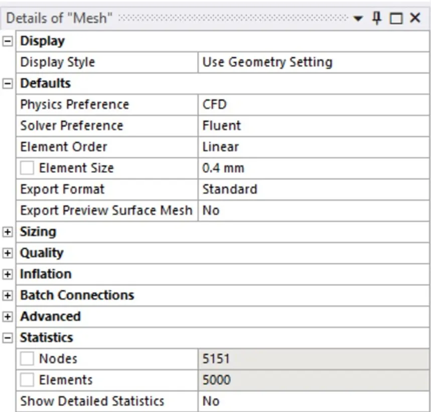
Residuals:
Time steps size [s] – 0.01
Number of Time Steps - 100
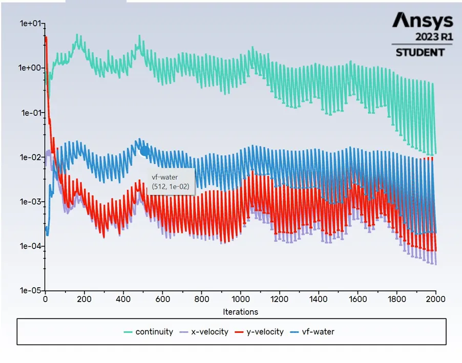
Volume of Fractions: (Water)
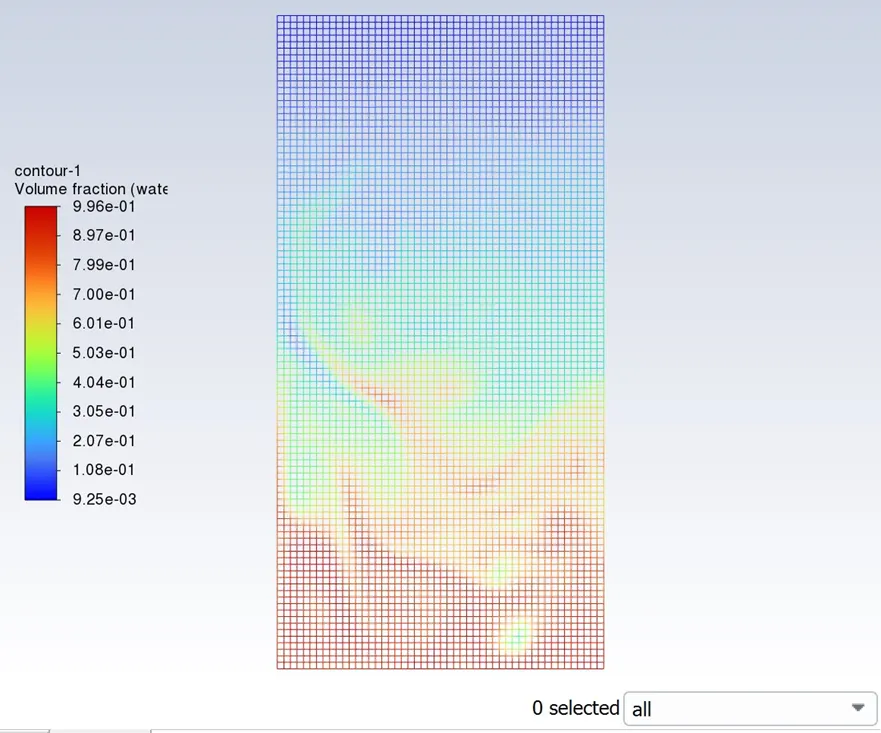
Solution Animation:
https://drive.google.com/file/d/1xOjHXG48hJo2hM0ZWzZmfpQGWbYH0Lx0/view?usp=sharing
3. Run one more simulation with water and user-defined material(density = 400 kg/m3, viscosity = 0.001 kg/m-s) for refined mesh.
Certainly, to run an additional simulation with water and a user-defined material with a density of 400 kg/m^3 and viscosity of 0.001 kg/m-s, you can follow these steps:
1. Geomentry and Mesh :
<!-- [if !supportLists]-->· <!--[endif]-->If you are using the same geomentry as in previous simuulations, ensure that the mesh is refines to the desired level, possibly smaller than the previous mesh sizes for improved accuracy. The mesh refinement should be fine near the fluid interface.
2. Material Properties:
<!-- [if !supportLists]-->· <!--[endif]-->Define the material propereties for both water and the user-defined material:
<!-- [if !supportLists]-->o <!--[endif]-->Water: Density = 998.2 kg/m^3, Viscosity = 0.001 kg/m-s ( if not already set)
<!-- [if !supportLists]-->o <!--[endif]-->User-Defined Material = ( eg., “CustomFluid” ): Density = 400 kg/m^3, Viscosity = 0.001 kg/m-s.
3. Solver Setup:
<!-- [if !supportLists]-->· <!--[endif]-->Configure the CFD solver, specifying the properties of the two fluids (water and the custom fluid) in the simulation setting.
4. Time Integration:
<!-- [if !supportLists]-->· <!--[endif]-->Set up transient simulations to capture the dynamic behavior of the fluids, just an previous simulations.
5. Post-Processing:
<!-- [if !supportLists]-->· <!--[endif]-->Analyze the results using post – processing tools to observe the behavior of the Rayleigh-Taylor instability and the interaction between water and the custom fluid.
5. Atwood Number Calculation:
<!-- [if !supportLists]-->· <!--[endif]-->Calculate the Atwood number for this case, which represents the density difference between water and the custom fluid.
A = (rho custom – rho water/ rho custom + rho water)
Subsitute the densities of the custom fluid and water to find A.
6. Analysis:
<!-- [if !supportLists]-->· <!--[endif]-->Intrepret the results and compare them to previous simulationswith just water. Observe how the variation in Atwood number affects the behavior of the Rayleigh – Taylor instability in this new scenario.
Case 3 User Defined Mesh & Water
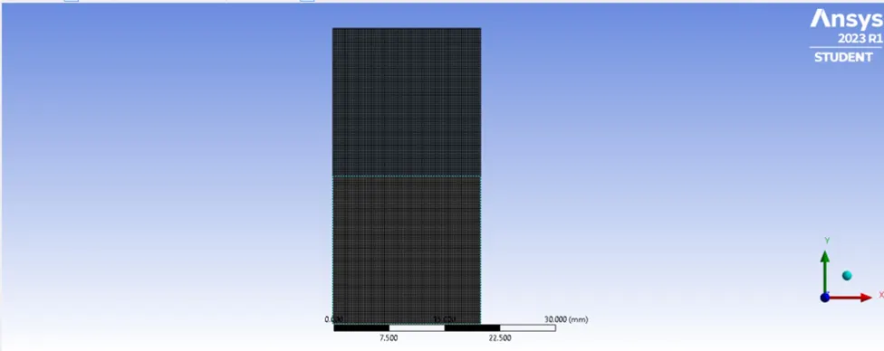
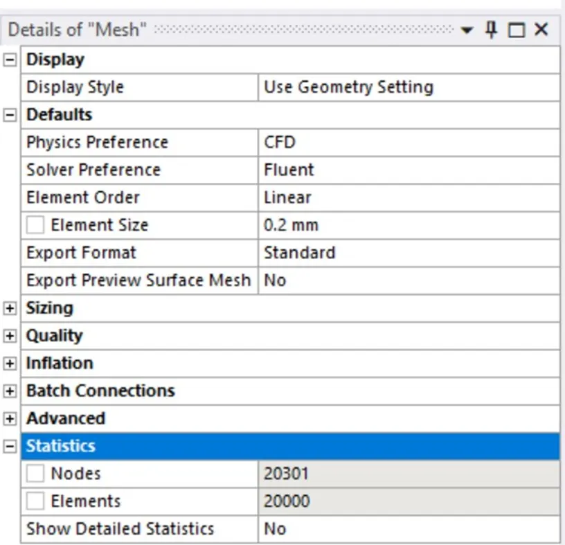
<!-- [if !supportLists]-->· <!--[endif]-->Base Mesh Size – 0.2mm
<!-- [if !supportLists]-->· <!--[endif]-->Number of elements – 20000
Mesh
<!--[endif]-->
<!-- [if !supportLists]-->· <!--[endif]-->The User Defined mesh of 0.2mm has been updated.
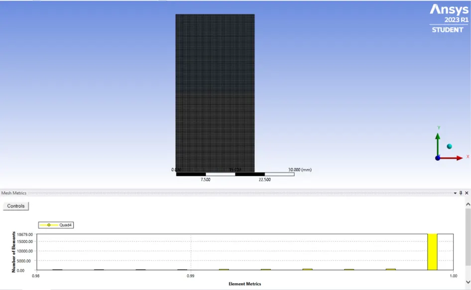
<!-- [if !supportLists]-->· <!--[endif]-->This plot show s the quality of the User Defined Mesh.
<!--[endif]-->
Set-up:
Material Properties
Air
<!--[endif]-->
Water
<!--[endif]-->
<!-- [if !supportLists]-->· <!--[endif]-->Here the Density and Viscosity value has been changed for the Water.
4. Multi-phase Model
<!--[endif]-->
Phases Phase Setup
Air - Primary Phase – Air
Water - Secondary Phase – Water
5. Patch
<!--[endif]-->
<!-- [if !supportLists]-->· <!--[endif]-->Intialization has to be done before patching the surfaces.
<!-- [if !supportLists]-->· <!--[endif]-->Phase
<!-- [if !supportLists]-->o <!--[endif]-->Water
<!-- [if !supportLists]-->· <!--[endif]-->Variable
<!-- [if !supportLists]-->o <!--[endif]-->Volume Fraction
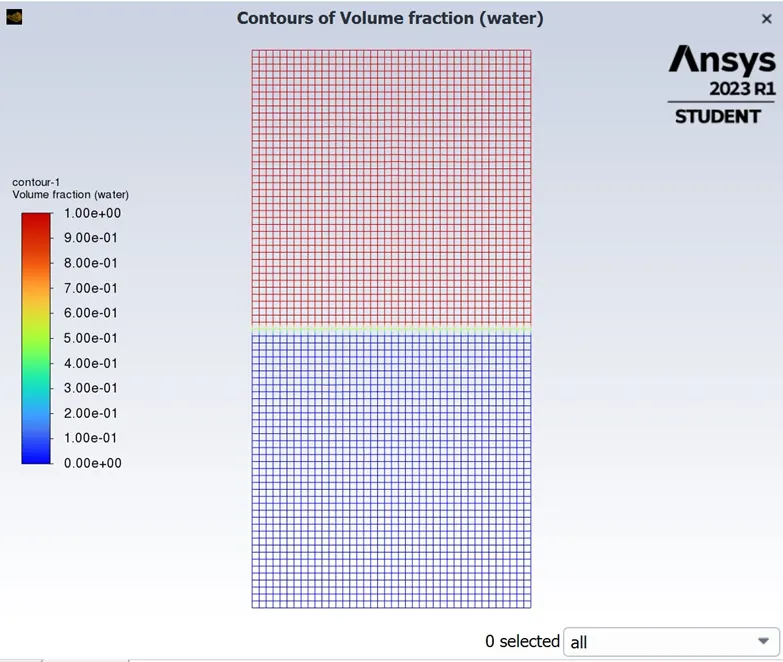
<!-- [if !supportLists]-->· <!--[endif]-->Zones to patch Value
<!-- [if !supportLists]-->o <!--[endif]-->Air surface - 0
<!-- [if !supportLists]-->o <!--[endif]-->Water surface - 1
<!--[endif]-->
<!-- [if !supportLists]-->· <!--[endif]-->This plot shows the patched surfaces between Air and Water.
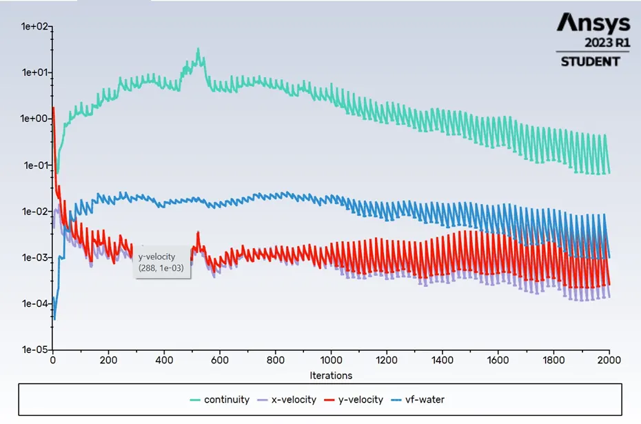
Residuals:
Time steps size [s] – 0.01
Number of Time Steps - 100
<!--[endif]-->
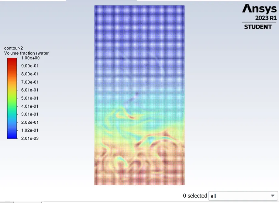
Volume of Fractions: (Water)
<!--[endif]-->
Solution Animation:
https://drive.google.com/file/d/19WyCJlwNz6oi2zGqcYyH-cEjBfqETy7p/view?usp=sharing
<!--[endif]-->
4. <!--[endif]-->Define the Atwood Number. Find out the Atwood number for both the cases and explain how the variation in Atwood number in the above two cases affects the behavior of the instability.
The Atwood number, denoted as “A,” is a dimensionless number used in fluid dynamics to characterized the behavoir of fluid flows with density differences. Its is particularly important in the study of buoyancy - driven flows, such as those that occur in natural convection, Rayleigh-Taylor instability, and various industrial processing involving fluids of different densities. The Atwood number quantifies the relative density differences between two fluids and is defines as follows:
A = (rho1- rho2)/(rho1+ rho2 )
Where,
<!-- [if !supportLists]-->a. <!--[endif]-->A is the Atwood number.
<!-- [if !supportLists]-->b. <!--[endif]-->Rho1 is the density of the lighter fluid.
<!-- [if !supportLists]-->c. <!--[endif]-->Rho2 is the density of the heavier fluid.
Let’s assume we have:
<!-- [if !supportLists]-->· <!--[endif]-->Rho1 = 400 kg/m^3 (density of the lighter fluid)
<!-- [if !supportLists]-->· <!--[endif]-->Rho2 = 1.225 kg/m^3 (density of the heavier fluid)
Now, plug thee values into the formula:
Case 1 Air + Water
Rho1 = 998.2, Rho2 = 1.225
A = (998.2 – 1.225)/(998.2+1.225)
Calculate the numerator and denominator:
A = (996.975/999.425)
A = 0.997
Case 2 Water + User Defined Material
Rho 1 = 998.2 Rho = 400
A = (998.2 – 400)/(998.2+400)
A = (598.2/1398.2)
A = 0.427
The differences in the fluid densities divided by their sum is defined as the Atwood number A.
The Atwood number measures the degree of density stratification between the two fluids. If A is positive, it indicates that the lighter fluid is on the top of heavier fluids, and if A is negative, it means the heavier fluid is on top.
CONCLUSION
In conclusion, the simulationof Rayleigh – Taylor instability is a complex computational endeavour that requires careful consideration of several key factors.
<!-- [if !supportLists]-->· <!--[endif]-->First, the choice of mesh size is pivotal. Smaller mesh size are essential for capturing the finer details and intricates of the instability, providing a more accurate representation of phenomenon like vortices, turbulent structures, and mixing pattern. Converserly, larger mesh sizes may compromise the simulation’s ability to resolve these crucial features. Therefore, when aiming for precision and fidelity in Rayleigh – Taylor simualtions, opting for smaller mesh sizes is a prudent choice.
<!-- [if !supportLists]-->· <!--[endif]--> Furthermore, ot’s important to recognize that Rayleigh – Taylor instabilities are inherently unsteady phenemenona. They involve dynamic and evolving fluid interfaces, making steady – state approaches unsuitable. Employing unsteady simulations is necessary to accurately capture the changing nature of the instability, including its growth and development over time.
<!-- [if !supportLists]-->· <!--[endif]-->Lastly, the Atwood Number, a dimensionless parameter characterizing density differences between the two fluids, plays a crucial role in influencing the behavior of Rayleigh -Taylor instabilities. Higher Atwood numbers enhance the instability, leading to more pronounced mixing, while lower Atwood numbers tend to stabilize the interface between the fluids.
<!-- [if !supportLists]-->· <!--[endif]-->In summary, successful Rayleigh – Taylor instability simulations require careful consideration of mesh size, the use of unsteady approaches, and an understanding of the Atwood Number’s influence. By addressing these factors, researchers and engineers can gain valuable insights into this complex fluid phenomenon and its applications in various fields, from astrophysics to engineering.