Week 4 - CHT Analysis on Exhaust port

       CHT ANALYSIS ON EXHAUST PORT

1. Give a brief description of why and where a CHT analysis is used.
2. Maintain the y+ value according to the turbulence model and justify the results. 
3. Calculate the wall/surface heat transfer coefficient on the internal solid surface & show the velocity & temperature contours in appropriate areas.
4. How would you verify if the HTC predictions from the simulations are right? On what factors does the accuracy of the prediction depend on?

1. What is CHT Analysis, Why and where it is used?

 

Conjugate Heat Transfer (CHT)  refers to the coupling of conduction in solids with the convective and radiative heat transfer in the surrounding fluids. In other words, CHT corresponds with the combination of heat transfer I solids and heat transfer in fluids. In solids, conduction often dominates whereas in fluidsm convection usually dominates. Efficiently combining heat transfer in solids is the key to designing effective heaters, coolers, or heat exchangers. Heat transfer in solids heat transfer in fluids are combined in majority of applications. This is because fluids flow around the solids, or between solid walls, and because solids are usually immersed in a fluid.

The CHT Anlysis is used in process which involve variations of temperature within solids and fluids, due to thermal interaction between solids and fluids. The exchange of thermal energy between the two physical bodies is called study of Heat Transfer, the rate of transferred heat is directly proportional to the temperature difference between the bodies. A typical example is the heating or cooling of a solid object by the flow of air in which it is immersed.

2. Maintain the y+ value according to the turbulence model and justify the results.

Maintaining an appropriate y+ value is crucial in Computational Fluid Dynamics (CFD) simulations, especially when using turbulence models. The y+ value represents the dimensionless distance from the wall to the first grid point in the computational domain, normalized by the molecular viscous length scale. It is used to ensure accurate representation of the near-wall flow behaviour and is closely related to  the accuracy of turbulence modelling.

Different turbulence models have varying requirements for the y+ value to accurately predict flow characteristics, such as well shear stress, skin friction, and heat  transfer. The choice of turbulence model (eg., k-epsilon, k-omega, SST, etc.) often determines the appropriate y+ range.

Here are a few common turbulence models and their corresponding y+ requirements:

• k-epsilon Model:
  • High-Reynolds-Number (HRN) version: y+ should be around 30.
  • Low-Reynolds-Number (LRN) version: y+ should be around 1.

• k-omega SST Model:
  • Typically works well in the range of 1

• Spalart-Allmaras Model:
  • Recommended y+ range is between 30 and 300.

Maintaining an appropriate y+ value is essential for several reasons:

1. Boundary Layer Resolution:

The y+ value ensures that the first grid point lies within the viscous sublayer or the buffer layer of the boundary layer. This is critical for capturing the near-wall turbulence behaviour accurately.

2. Turbulence Modeling Accuracy:

Turbulence models are based on certain asumptions and are designed to work effectively within specific flow regimes. By maintaining the appropriate y+ value, you ensure that the model’s assumptions are valid and the resulting predictions are accurate.

3. Wall Shear Stress and Heat Transfer:

Accurate prediction of wall shear stress and heat transfer rates relies on correctly modeling the flow behaviour near the wall. A proper y+ value helps achieve this accuracy.

4. Convergence and Stability:

Using an appropriate y+ value can improve the convergence and stability of simulations. Incorrect y+ values can lead to convergence issues and unphysical results.

To justify the results obtained with a particular y+ value, you should follow these steps:

1. Validation:

Compare your simulation results with experimental or benchmark data for similar cases. If your results are in good agreement, it’s an indicator that your chosen  y+ value is appropriate.

2. Grid Sensitivity Analysis:

Perform a grid sensitivity analysis by varying the grid resolution and observing how the results change. This can help identify whether your chosen y+ value is providing consistent and convergent solutions.

3. Physical Interpretation:

Check if the predicted flow behaviour matches your understanding of the physics. If the flow pattern near the wall is consistent with the expected behaviour (eg., Velocity profiles, boundary layer growth), it’s positive sign.

4. Sensitivity to y+ Variation:

Asses how sensitive your results are to changes in the y+ value. If the remain relatively stable within a  reasonable y+ range, it suggests that the chosen value might be appropriate.

3. Calculate the wall/surface heat transfer coefficient on the internal solid   surface & show the velocity & temperature contours in appropriate areas.

Calculating the wall heat transfer coefficient (HTC) involves determing the rate of heat transfer per unit area from the fluid to the solid surfaces. The heat transfer coefficient is given by Newtons’s Law of Cooling.

q = h. (Tf – Ts)

Where:

• q is the heat transfer rate per unit area (W/m^2 ).
• h is the heat transfer coefficient (W/m^2.K).
• Tf is the fluid Temprature (K) at the solid-fluid interface.
• Ts is the solid surface temperature (K).

The heat transfer coefficient  h depends on the fluid properties, flow conditions, and geomentry of the system. Commonly, it’s determined using empiricial correlations or simulations.

To calculate and visualize the velocity and temperature contours in appropriate areas, you typically perform Computational Fluid Dynamics (CFD) Simulations. In this case, I can guide you through the general steps:

1. Geomentry and Meshing:

Create or import the 3d geomentry of your system, including the solid surfaces. Generate a mesh that adequately resolves the boundry layers and regions of interest, like near-wall regions.

2. Boundary Conditions:

Define boundary conditions including fluid Inlet and Outlet conditions, wall boundary conditions, Initial conditions, and turbulence models.

3. Solver Setup:

Choose a CFD solver and setup the simulation parameters such as time step size, convergence criteria, and solver settings.

4. Run Simulation:

       Run the simulation to obtain velocity and temperature distributions within the fluid domain.

5. Post-Processing :

  Once the simulation is complete, post-process the results. Most commercial CFD software packages provide tools for this purpose.

6. Heat Transfer Coefficient Calculation:
   • Extract the temperature at the solid-fluid interface (Tf) and the solid surface temperature (Ts) from the simulation results.
   • Calculate the local heat transfer rate per unit area (q) using the temperature difference.
   • Determine the heat flux (q/A) at each point on the solid surfaces.
   • Calculate the local heat transfer coefficient (h) using the heat flux, fluid properties, and temperature difference.
7. Visualization:

      Plot the velocity and temperature contours in the areas of interest, like near the solid   surface. Most CFD software allows you to generate contour plots and streamline plots.

4. How would you verify if the HTC predictions from the simulations are right? On what factors does the accuracy of the prediction depend on?

Verifying the accuracy of Heat Transfer Coefficient (HTC) predictions obtained from simulations involves comparing the simulation results to experimental or benchmark data. The goal is to assess how well the simulation captures the real-world heat transfer behavoiur. Here’s how you can verify the HTC predictions and the factors that influence the accuracy of the prediction.

Verification Steps:

                    

1. Experimental Data comparsion:

     Obtain experimental data for the same system or a similar case. This could include data for the same system or a similar case. This could include data from the literature, lab experiments or field measurements. Compare the simulated HTC values with the experiments data.

2. Statistical Metrices:

Calculate statistical metrices such as Mean Absolute Error (MAE), Root Mean Square Error (RMSE), or Coefficient of Determination (R^2) to quantitatively measure the agreement between simulation and experiment results.

3. Trend Analysis:

  Examine the trend of the HTC values across different simulation scenarios and experimental conditions. Ensure that the simulation captures the same as the experiments.

4. Sensitivity Analysis:

      Perform sensitivity analyses by varying key parameters, such as mesh resolution, boundary conditions, or turbulence models. Evaluate how these changes affect the predicted HTC values.

Factors Affecting Accuracy:

 

1. Grid Resolution:

A finer mesh near the wall is crucial for capturing boundary layer behaviour accurately. Inadequate resolution can lead to Incorrect HTC predictions.

2. Turbulence Modeling:

The choice of turbulence model affects the HTC, Select an appropriate turbulence model based on the flow characteristics.

3. Boundary Conditions:

Accurate specifications of boundary conditions, such as inlet velocity and temperature, is essential for reliable HTC predictions.

4. Geomentry and Mesh Quality:

The geomentry representation and mesh quality significantly influence the accuracy. Poor mesh quality or simplications in geomentry can lead to errors.

5. Physical Properties:

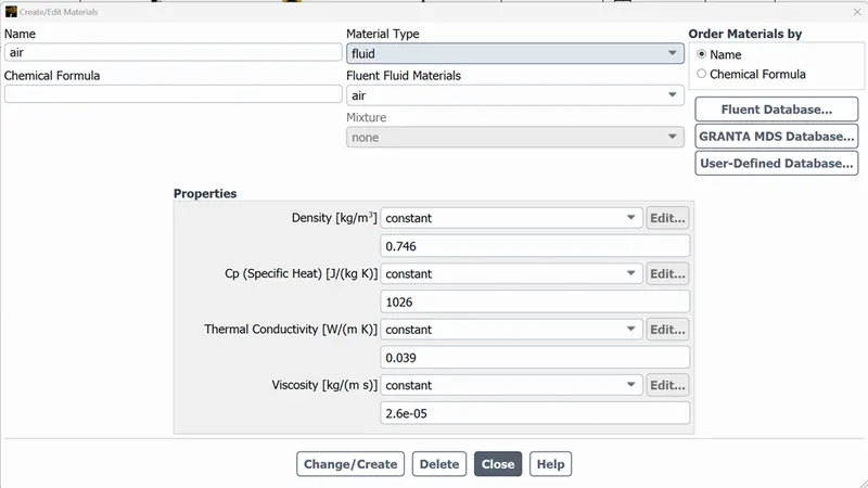
Accurate input of of fluid properties (Density, viscosity, specific heat) is critical for HTC calculations.

6. Solver Settings:

Numerical solver settings, such as time step size and convergence criteria, impact the accuracy of transient simulations.

7. Conduction and Radiation:

If there are conductive or radiative heat transfer effects, they need to be accurately modeled and accounted for.

8. Experimental Uncertainties:

Real-world experiments have uncertainties. Make sure to consider the measurement errors and uncertainties in experimental data when comparing with simulations.

9. Surface Roughness:

If the surface has roughness, it can influence the boundary layer behaviour and consequently affect the HTC predicions.

10. Geomentry Complexity:

Complex geomentrices might require more sophisticated modelling techniques, such as conjugate heat transfer, to accurately predict HTC.

11. Heat Flux Variation:

If the heat flux is not uniform along the surface, accurate prediction can be challenging.

12. Reynolds Number and Flow Regime:

HTC can vary with Reynolds number and flow regime. Make sure your simulation covers the appropriate range.

INTRODUCTION

          Here our objective is to simulate the flow through it as the flow is going through manifold it is going to exchange heat with the solid, we want to simulate that process. We are going to do this by initially assuming that the flow is coming through the exhaust which is basically through all the four inlets and we are giving to assume that the fluid is really very hot and that going to heat the solid pipe from inside and on the external surface we are assuming that there is a particular heat transfer. So in real world scenario as your engine is air cooled as it is exposed to air and air which is near to the port has particular heat transfer coefficient and that would be provided as input and theat value depends on the external air Reynolds number. We can simulate it and find the value but here we are just giving the value as input i.e, heat transfer coefficient for the outer wall boundary condition. Then by asking these assumptions into conisderation.

Solution Procedure

• We will simulate both fluid flow and also the heat transfer to the solid i.e., CHT analysis on an Exhaust port with the steady state. Then for solving we follow the below Procedure:

• Geomentry Setup
• Meshing
• Problem setup
• Solving
• Post Processing

• Then we calculate the wall/surface heat transfer coefficient on the internal solid surfaces & show the velocity & temperature contours is in appropriate areas.

Simulating the flow with the steady case:

In the ANSYS work bench we first open the fluent module by drag and drop. The we follow the procedure we have mentioned above.

1. Geomentry setup:

• In fluent module we have to open SpaceClaim and import the geomentry.

 

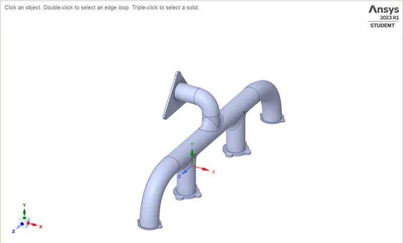
• If you look closely to the geomentry it has solid part. So first let us extract the fluid volume. For that we have to go to,

                     Prepare à Volume Extract à Select edge selection à then select all edges of inlet and outlet à Then click ok. Fluid volume will be created.

 

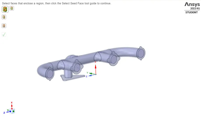
• Then after the volume has created then in the design change the name of the components i.e., fluid volume to fluid and solid volume to solid.
• After changing the components, We should have both of the volume overlap perfectly, inorder to fix that we need to share to opology.
• In order to do that the work as one component we need to make sure that share to opology is set to share. Only then these two individual blocks going to exchange information i.e., the meshing is going to uniform and with perfect connectivity. So we need to fix this.

Share to opology

 

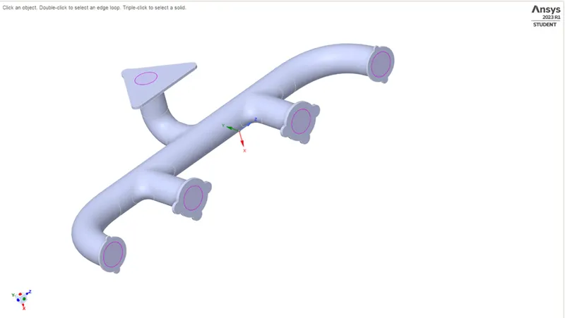
• For that in properties enable share for share topology, But before that we need to do important step to follow. We need to take two volumes and move into a new component, and this is the final geomentry which consists of solid volume and fluid volume and then delete the old empty components. Now enable the share to opology and then go work bench and click share. This is very important if you don’t do this step you will not see the single interface between them. So this is particular step takes care of creating the interfaces, so that you will have one interface between your solid volume or block and fluid block. Once you have done this you will see the pink circles at the interface, that basically tells you where the things are being shared. Basically what this means is that you will have a sharing between inner wall of solid and outer layer of fluid will have a common interface and bounds of share is one. This is only interface you will see.
• Now if you open meshing and you will see that there is perfect mesh connectivity and the interface is shared perfectly. This is exactly how we need to make meshes for CHT simulation.
• This completes the creation of geomentry. Then we close the SpaceClaim.

2. Meshing:

• For meshing we open Meshing, where we mesh our model so that we can use it to solve our model.

 

Case1 Baseline mesh

• Base Mesh Size - 200
• Y+ value - 5
• First cell height – 0.6 mm
• Number of inflation layers – 12
• Growth Rate – 1.25
• Total boundary layer thickness - 0.8mm
• Number of elements - 252182

Mesh

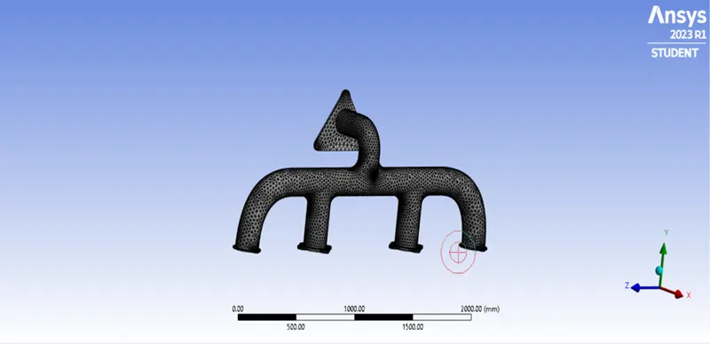
• In general it is always good to name the surfaces before meshing. So let us do that.
• We first select the entity by using the entity selection by using faces so that we can provide name for our entity selection.

                        Steps: select the edge you want to name using edge selection à then press N à Name the selection.

• In the similar way we name our inlets, outlet and for outer face just double click on the outer part anywhere and ANSYS mesher will automatically select the faces we require and we name it ass outer wall convection ( Since we are going to use convective BC for it), and you can see additional walls like flangs which have not selected you and name them or even if you don’t name what ANSYS mesher will do is it going to automatically import those into fluent as a wall by default these walls will have adiabatic BC,which is exactly what we want.

Named Selections

 

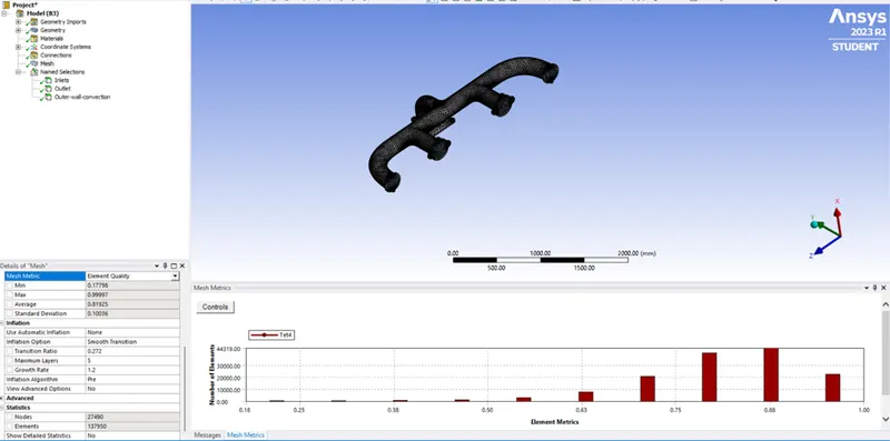
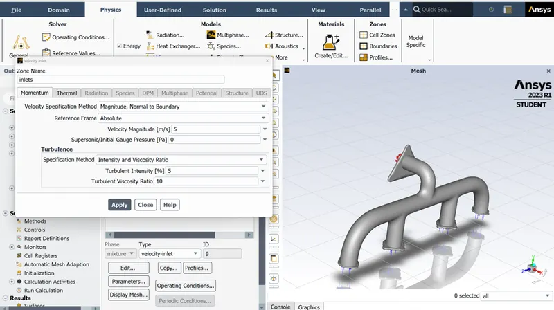
Inlet Boundary Condition (velocity inlet) @ 5m/sec.

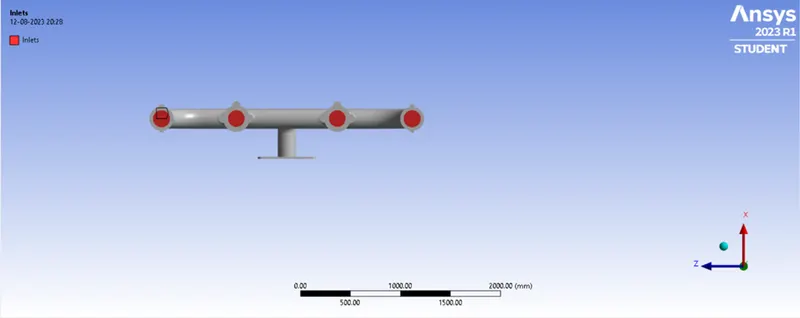
This plot shows the Inlet on the Exhaust port.

 

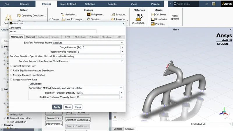
Outlet ( Pressure outlet) Gauge pressure 0Pa

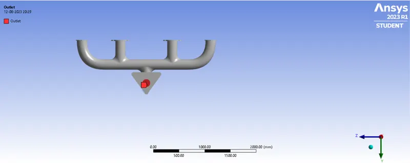
This plot shows the Outlet on the Exhaust port.

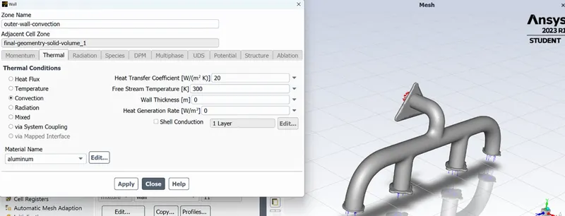
Outer wall Convection (Heat transfer coefficient 20(W/m^2k) free stream temperature 300K)

The flanges atound the inlet and the component encompassing the outlet are adiabatic ( no heat transfer takes place through these walls).

• Then next thing to do is to mesh. We click the mesh option in the side window and create our base line mesh. We then refine mesh. Let’s mesh the geomentry. Once the mesh has done we need to see what are the things we have to refine. Let us free refine one by one. Let us start with creating inflation layer.

                Inflation Layer:

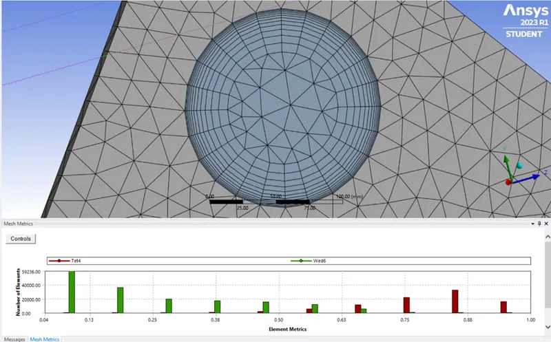
• Inflation layer helps us to create a body fitted mesh. It means it creates a layer of mesh same as the geomentry.
• Since at the interface it is very important and we want to calculate the heat transfer at that place we need to take that region and create inflation layers so that flow is captured exactly and the values are calculated exactly.
• To do this we first with selecting fluid part and naming it as inflation layer.
• In the global mesh select inflation option and in that for use automatic inflation – select all faces in the choosen named selection and for named –  select the inflation layer which we have just named.
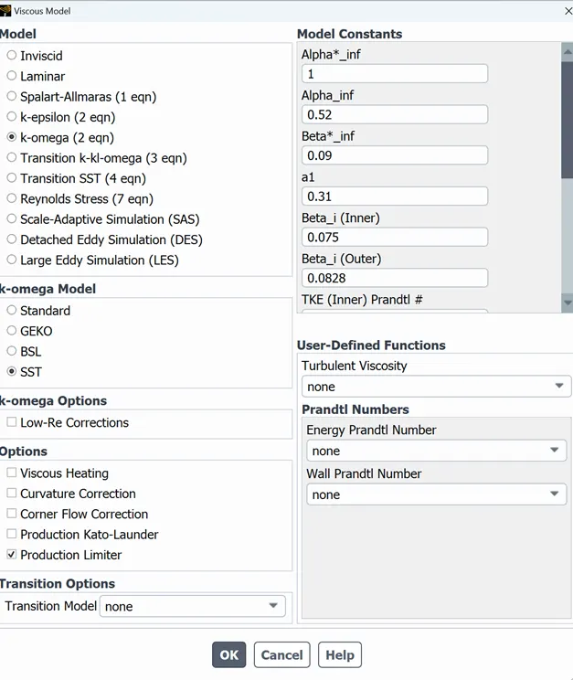
• And for inflation option we use first layer thickness and we give this based on y+ value and the turbulence model we use. Here we use k-omega SST turbulence model so y+ should be in between 0.1 to 5.

 

3. Set up:

The different boundary conditions are

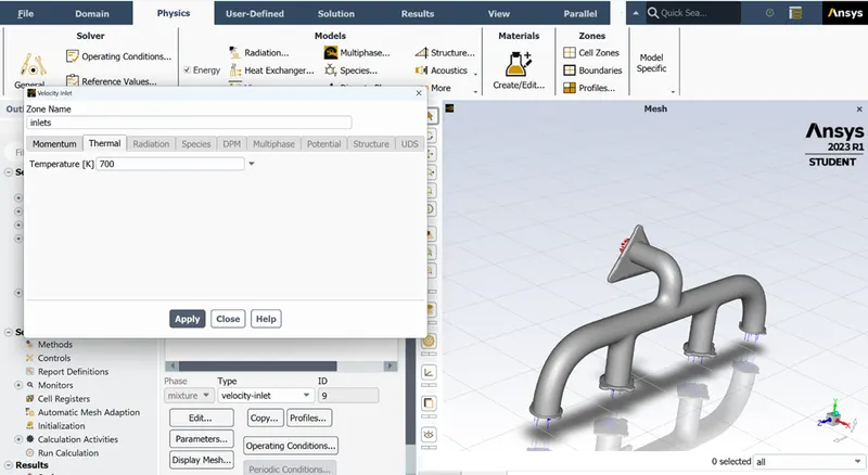
1. Inlet Boundary Conditions

• Velocity Inlet
• Velocity magnitude: 5 m/sec
• Temprature: 700K

 

 

 

 

2. Outlet Boundary Condition

• Pressure Outlet
• Gauge Pressure: 0pa

 

 

 

3. Outer wall Convection

• Wall
• Thermal condition: Convection
• Heat Transfer Coefficient: 20 (W/m^2k).

 

The rest boundary condition values are set up as default values in ANSYS - FLUENT.

4. Energy equation: It is turned on
5. Viscous Model:
6. Material Properties

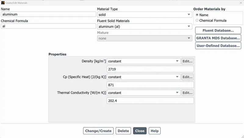
 Fluid

  Solid

 

 

 

 

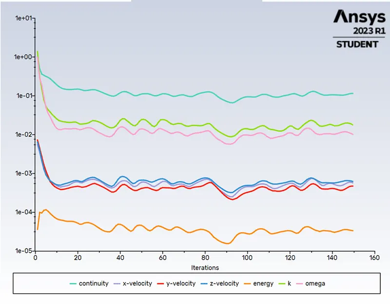
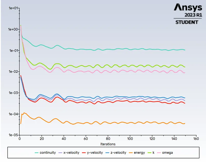
 Residuals plots

Number of iterations: 150

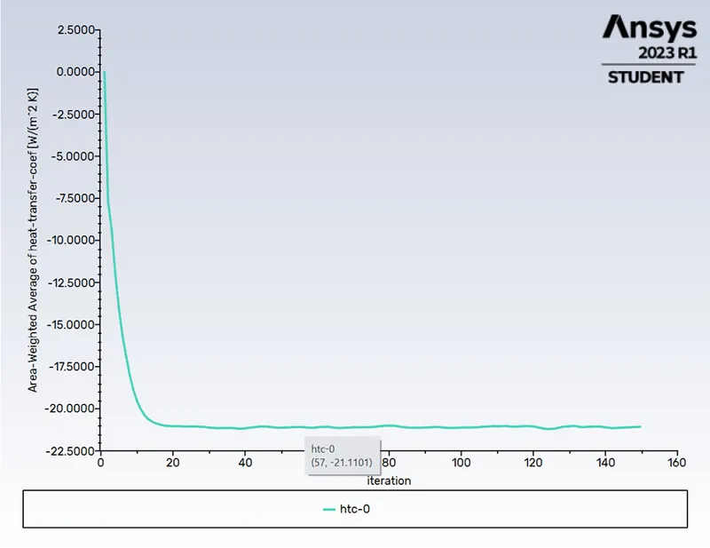
Heat Transfer Coefficient:

 

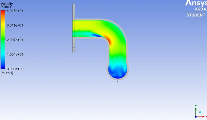
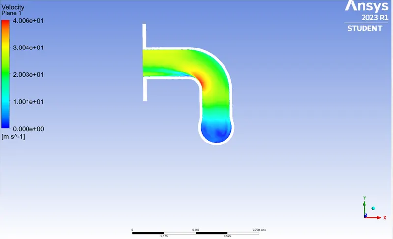
Velocity Plane

 

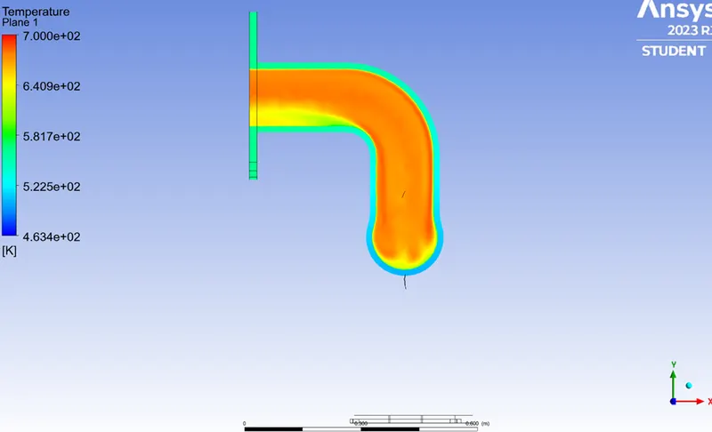
Temprature Plane:

 

 

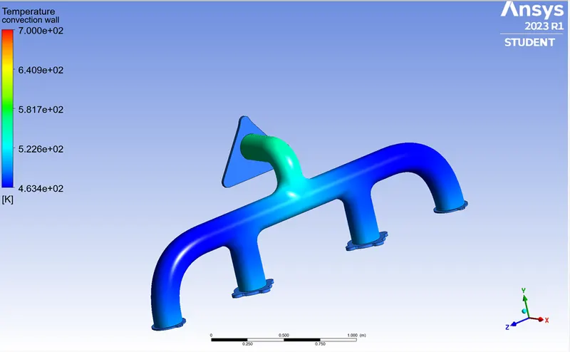
Temprature:

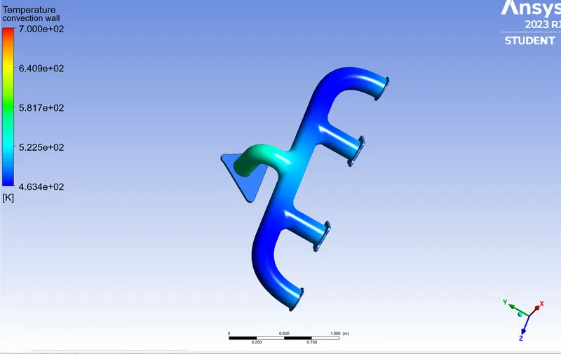
These are the plots of the temprature contour on the exhaust port.

 

 

 

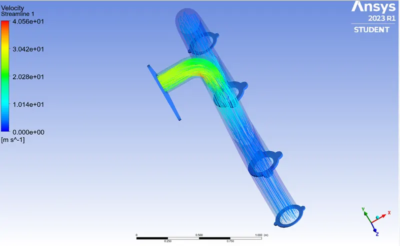
Velocity Streamline:

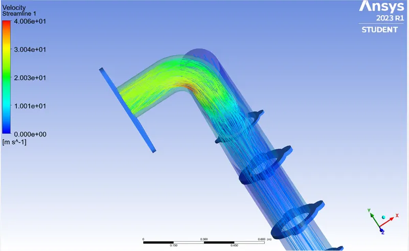
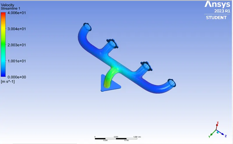
• Here in the below streamline plot you can see that streamlines coloured with velocity

 

 

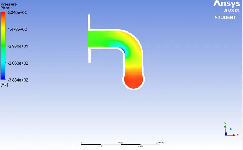
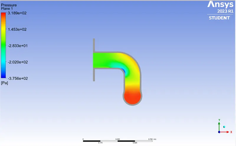
Pressure Plane:

 

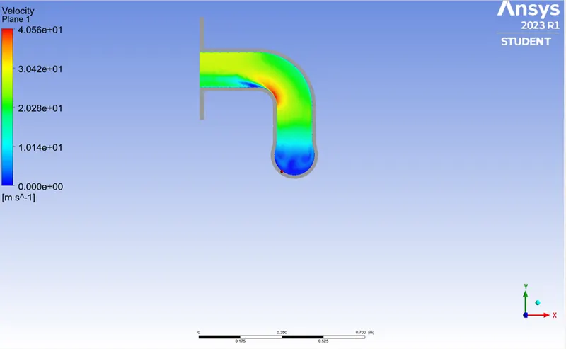
Velocity Plane:

 

 

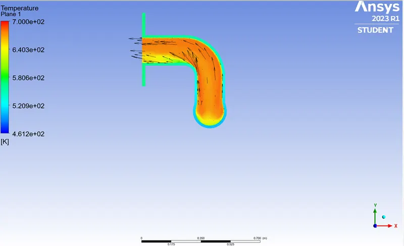
Temprature Vectors:

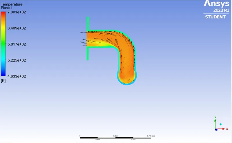
These plots that shows the vectors among Outet of the exhaust port.

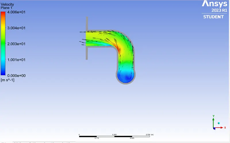
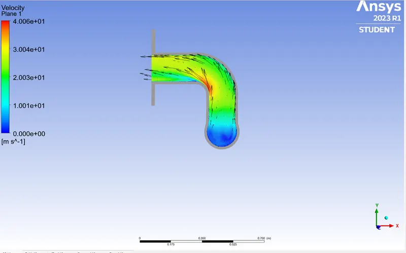
Velocity Vectors:

Heat Transfer Coefficient:

Case2 Refined mesh

• Base Mesh Size - 150
• Y+ value - 5
• First cell height – 0.5 mm
• Number of inflation layers – 12
• Growth Rate – 1.25
• Total boundary layer thickness - 8mm
• Number of elements – 257033

Residuals plots

Number of iterations: 150

 

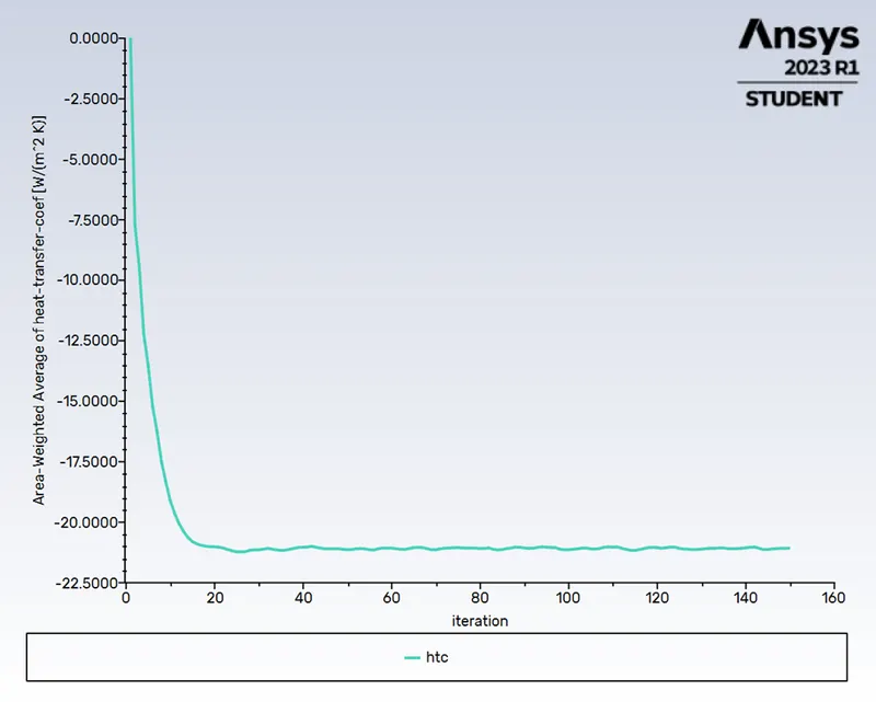
Heat Transfer Coefficient:

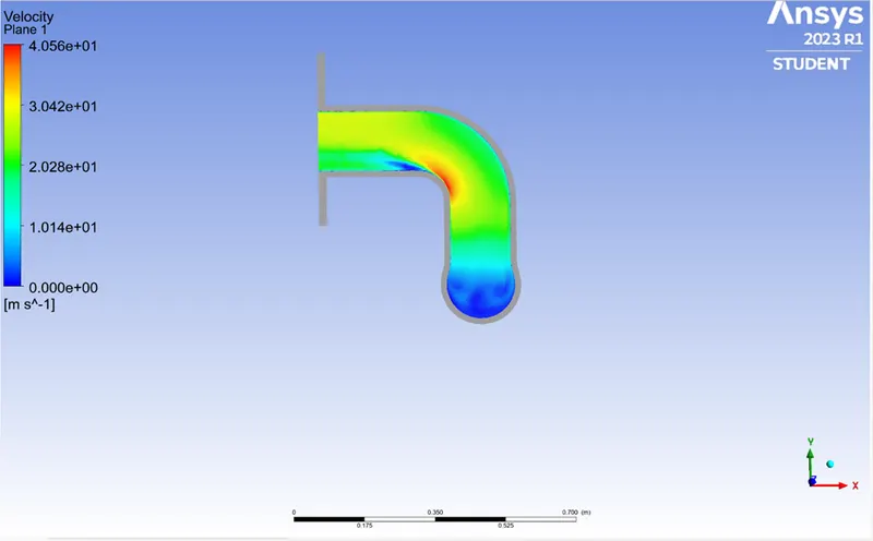
Velocity Plane:

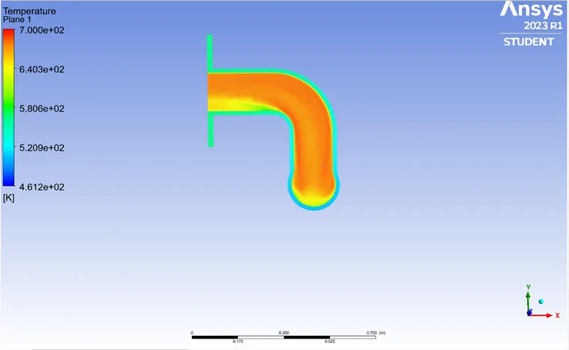
Temprature Plane:

 

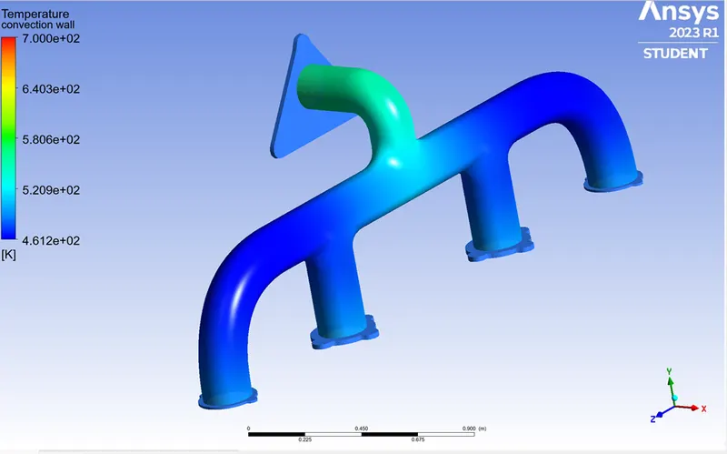
Temprature:

 

 

Velocity Streamline:

 

 

Pressure Plane:

 

Velocity Plane:

 

Velocity Vectors:

 

Temprature Vectors:

 

 

Heat Transfer Coefficient:

 

Conclusion:

In case mesh generated has default setting and the results captured are less accurate due to the same.

 From the above cases we notice the following results as -

• Velocity tends to increase from inlet to outlet due to mass conversation and mixing of air.
• Transfer of heat from fluid to solid is high and leads to formation high velocity at the junction resulting in HTC capturing.
• The internal flow velocity and its characteristic are affected by initial velocity, pressure and physical features of geomentry. Thus, CHT analysis is essential prior experimental process for better prediction product life of design component.
• As shown in the plots, the exhaust gases passing through the manifold transfers some of the heat via convection. The amount of heat transfer can be releated directly with the velocity of exhaust.
• The temperature is lower where flow stagnates or is moving at the velocity. As the velocity increases, so does the Reynolds’s number and the amount of heat transfer.