Week 2 - Flow over a Cylinder.

Objective

Stimulate the flow over a cylinder and explain the pharma of karmen Vortex Street.

Part 1

Stimulate the flow with steady and unsteady case and calculate the Strouhal Number for Re= 100.

Part 2.

Calculate the coefficient of drag and lift over a cylinder by setting the Reynolds number to 10,100,1000,10000& 100000. (Run with steady solver)

Discuss the effect of Reynolds number on the coefficient of drag. [Results should be validated with any standard literature and error should be within 5 %]

Expected results

1. In both approaches, Show that the flow as converged. This is what quantities are cloths need to be look at to determine that the flow as converged?
2. Plots of the coefficient of drag and lift
3. Plots to show Vortex shedding Shedding behind the cylinder.
4. Mention the preferred material at the end of the challenge submission page.

Introduction:

Vortex shedding is an oscillating flow that Takes place when a fluid such as air or water flows past a bluff (as opposed to streamlined) body at a certain time velocities, Depending on the size and shape of the body. In this flow, vorties are created at the back of the body and detach periodically from either side of the body, forming a von Karmen Vortex Street. The object will tend to move towards the low pressure zone. Moreover, von Karmen vortex Street is a repeating pattern of swirling vortices, caused by a process known as vortex shedding, HS responsible for the unsteady separation. Separation of flow of a fluid around blunt bodies.

Strouhal number:

The Strouhal number Is here dimensionless number describing oscillating flow mechanisms

Strouhal number is often given as

St = fL/U,

Where f is the frequency of vortex shedding

L is the characteristic length

U is the flow velocity

Geometry:

We used line tool to draw with dimension:

Cylinder dia 2m, with circle orgin - -20 on x and +40 on x – axis box – 60x20m

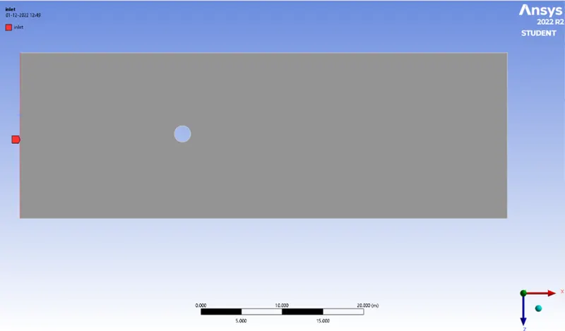
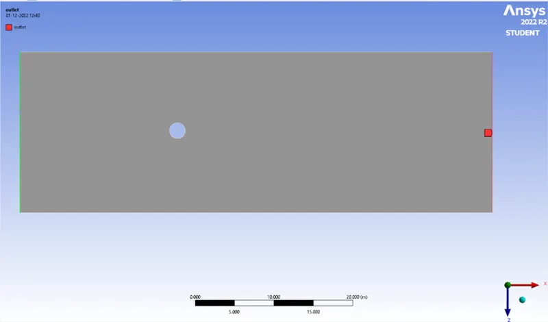
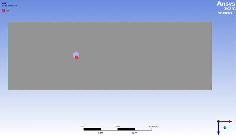
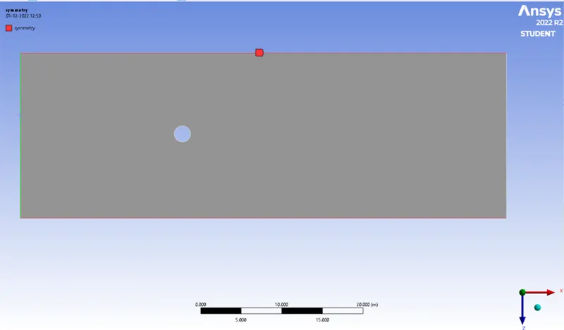
An Infinitely long. Circular cylinder of diameter D = 2.0m is placed in an otherwise undistributed uniform crossflow. The lateral boundry and the exit in the far wake are placed at 10 D and 20 D from the centre of the cylinder, respectively. The cylinder is used to drawn in spaceclaim.

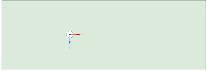
Converting the geomentry by using the command pull and select. Also, delete the inside the circle to carry out the simulation.

Then they select the construction line under the curves.

Mesh:

First of all, the baseline mesh autogenerated quad mesh was created. After that, it will change according to simulation requirements, and it was finely tuned with the help of triangular mesh generated. The midel meshed with an element of 0.

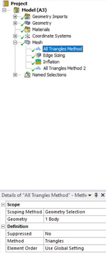
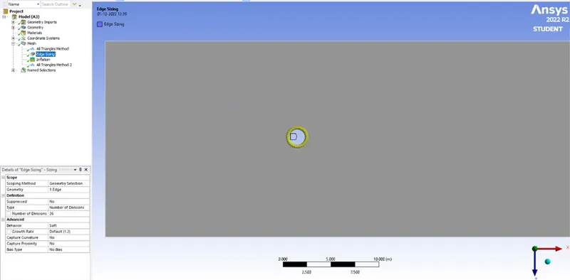
Edge sizing:

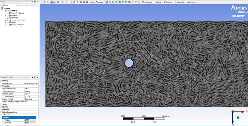
Boundry flagging:

Inlet:

Outlet:

Cylinder wall:

Symmetry:

Setting up physics, boundry conditions and output:

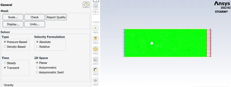
Solver: Unsteady Stare

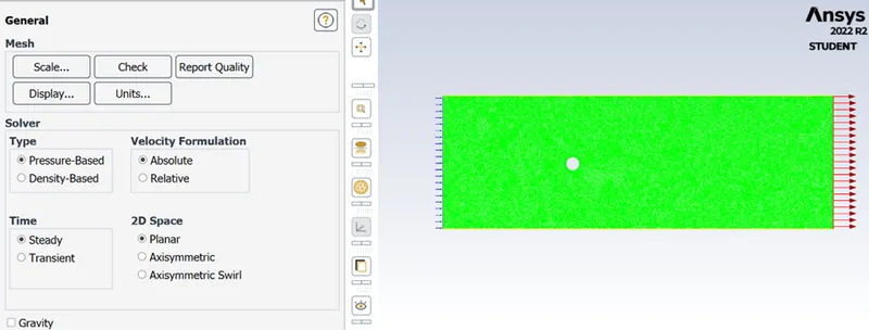
Steady State

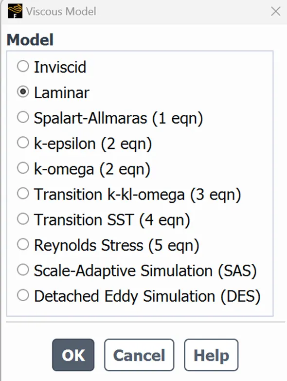
Viscous Model:

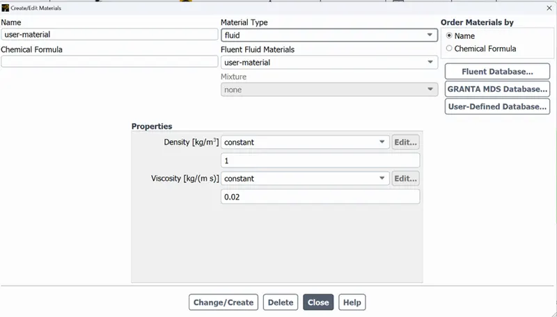
Material:

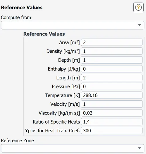
Reference Values:

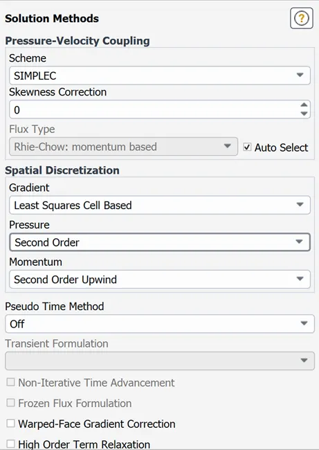
Solving method (Unsteady state):

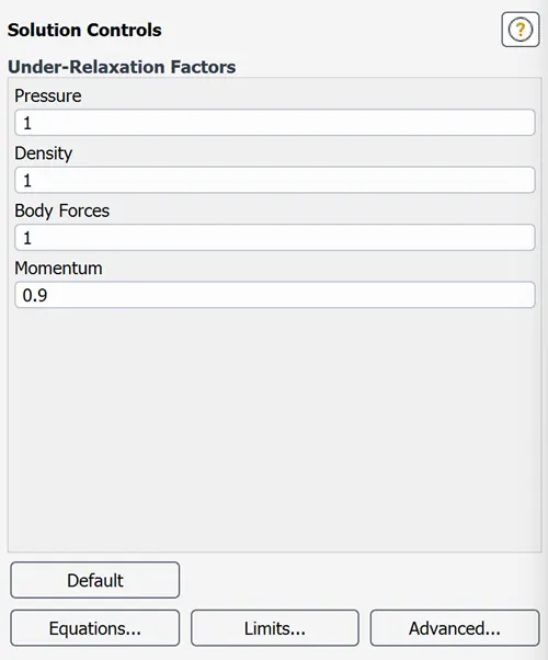
For velocity-pressure coupling, the SIMPLEC algorithm was used. When the SIMPLEC algorithm is used, the pressure under-relaxation is automatically increased to 1.0. The setting for under-relaxation is 0.3 (When the default SIMPLE algorithm is used). Here the momentum under-relaxation has also been increased from 0.7 to 0.9 to yield better convergence.

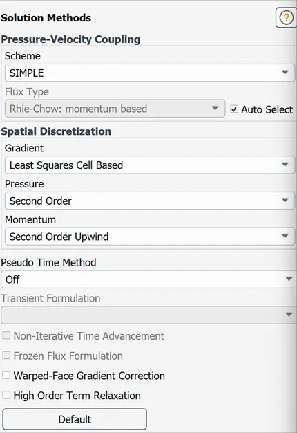
Steady state

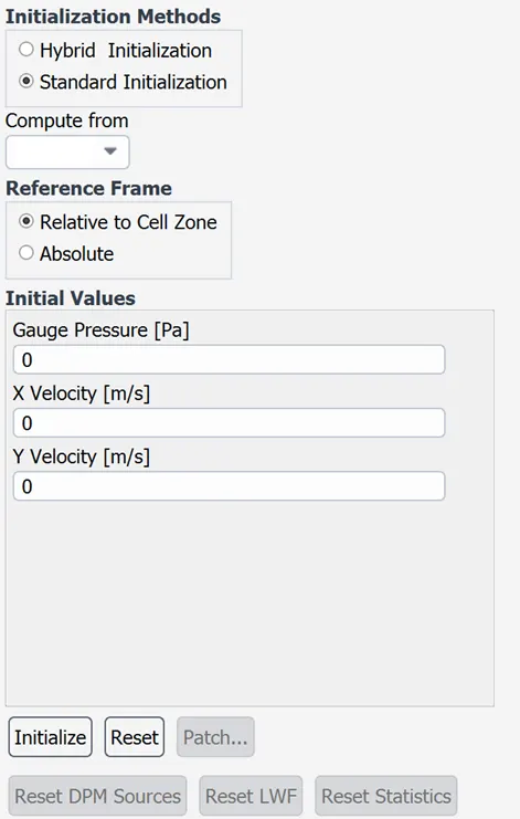
Solution Initialization:

Unsteady state:

Steady state:

Hybrid Initilization

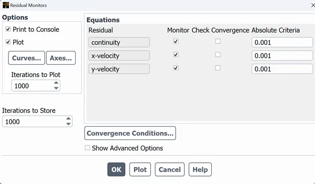
Residuals:

Animation:

Autosave: 1

Create the minimum using the solution command for the velocity it was up before running the simulation. Also, recorded for every 10 iterations.

Run Calculations:

Steady state:

1000 iterations

Unsteady state:

2000 iterations

Steady State Simulations:

The following plots to be shown for both steady and unsteady simulation

Plots:

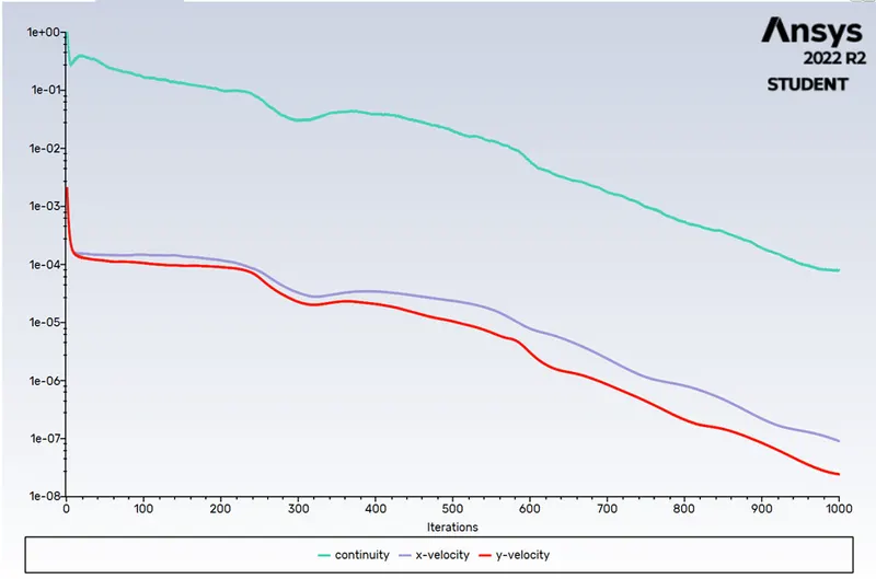
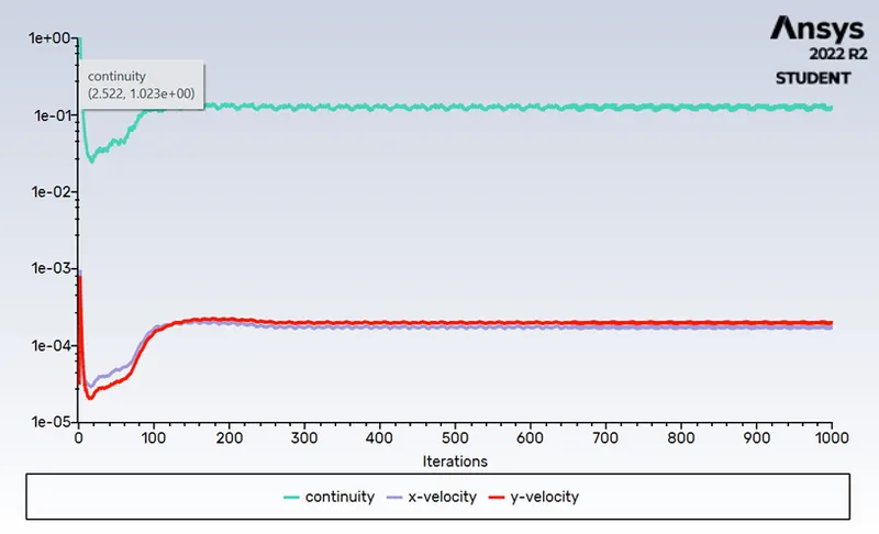
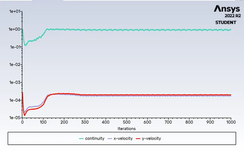
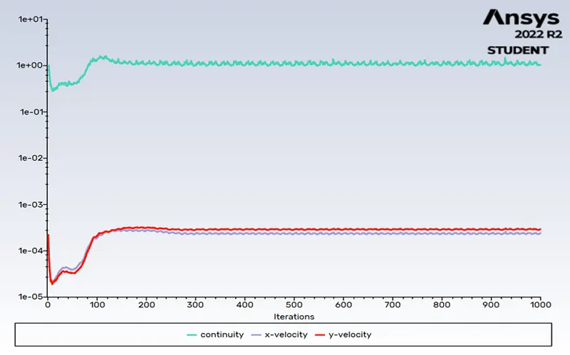
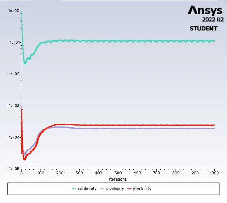
Residuals:

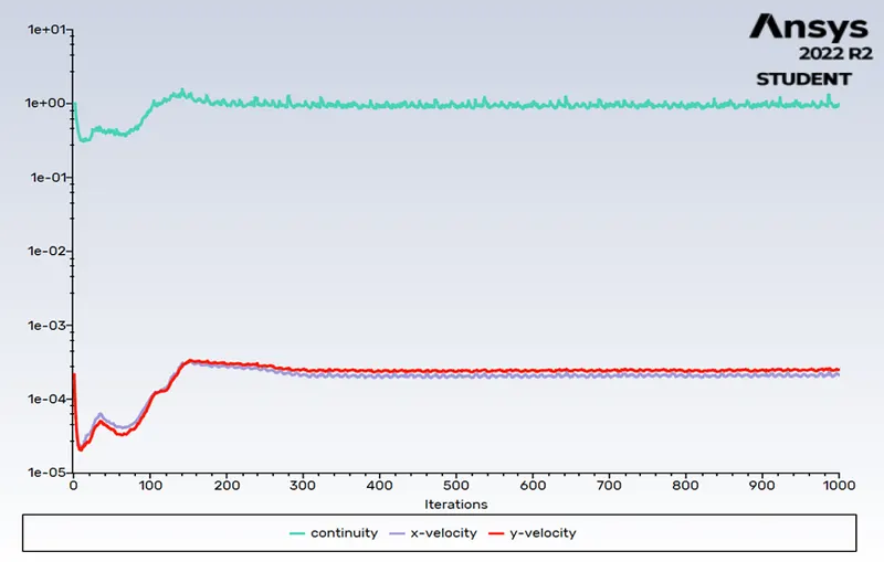
This plot shows at what point convergence has achieved.

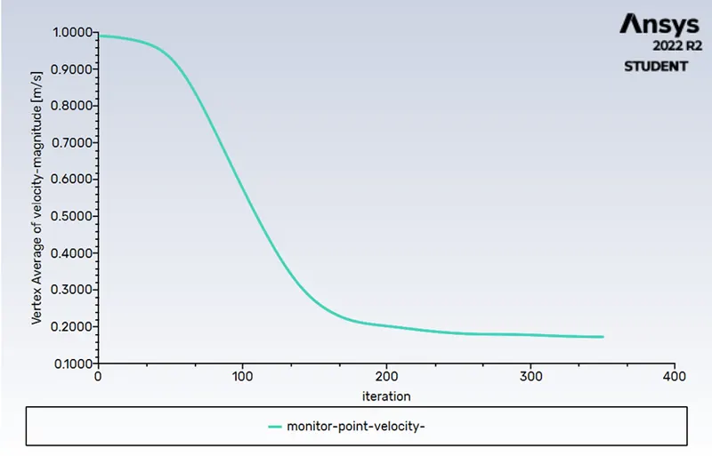
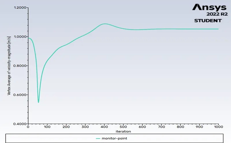
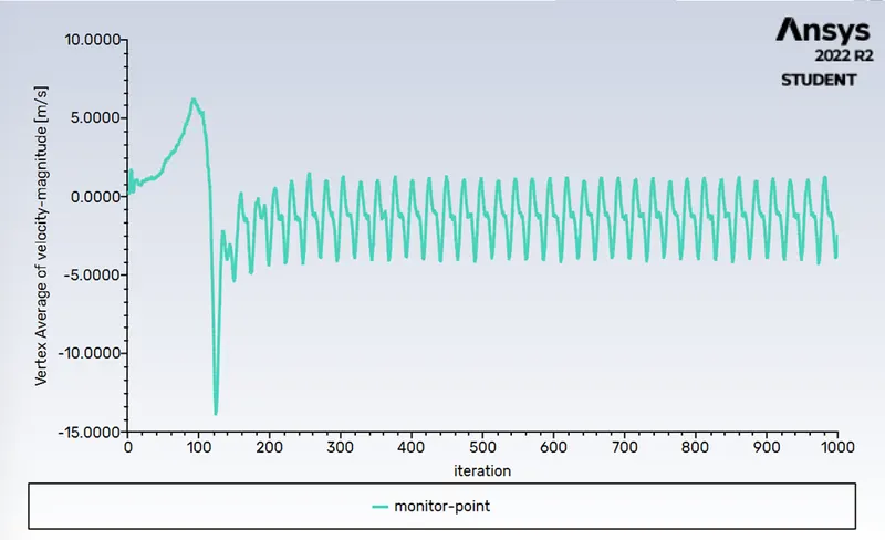
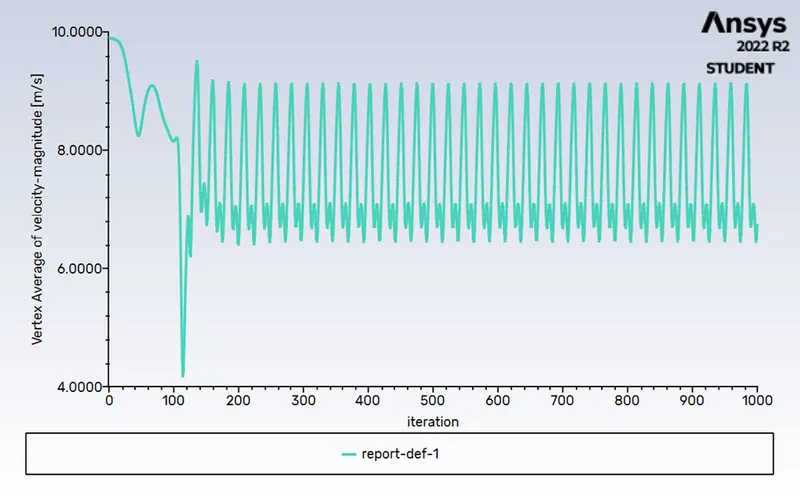
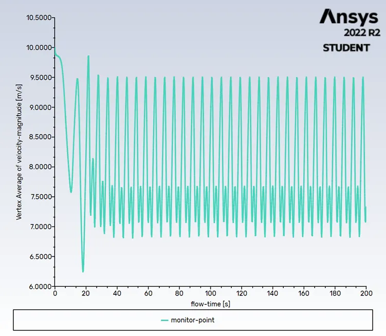
Monitor point velocity plot:

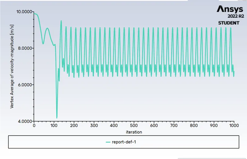
The monitor of 8m is placed at a distance from the cylinder to calculate the velocity from the point.

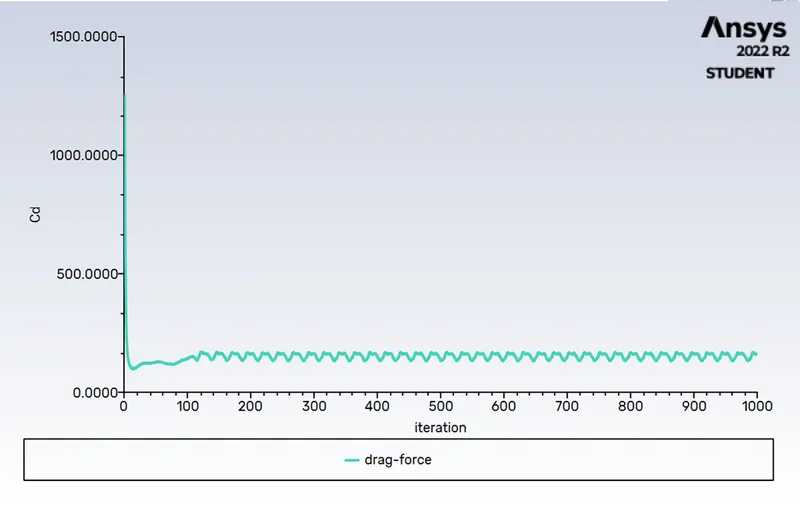
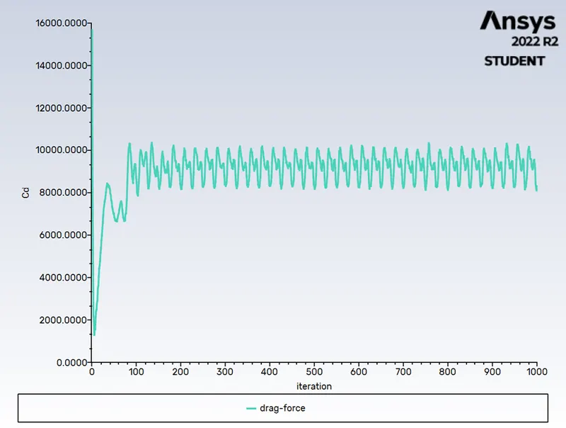
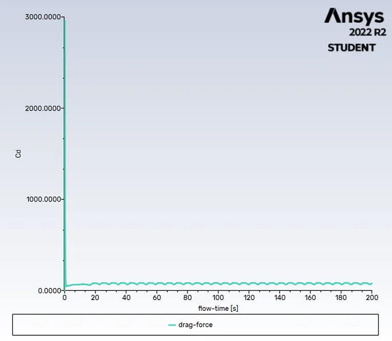
Drag Coefficient Plot:

To calculate the drag coefficient.

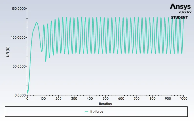
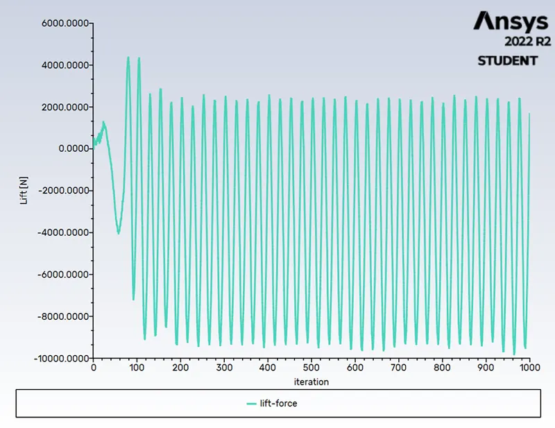
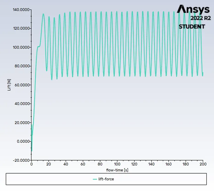
Lift Coefficient Plot:

To calculate the lift coefficient.

Velocity & Pressure Contour:

To see the velocity & pressure changes when flow past over a cylinder.

Case1:

Reynolds Number = 10

Viscosity = 0.02

Velocity = 0.1

Iterations = 1000

Residuals plot:

Monitor point velocity:

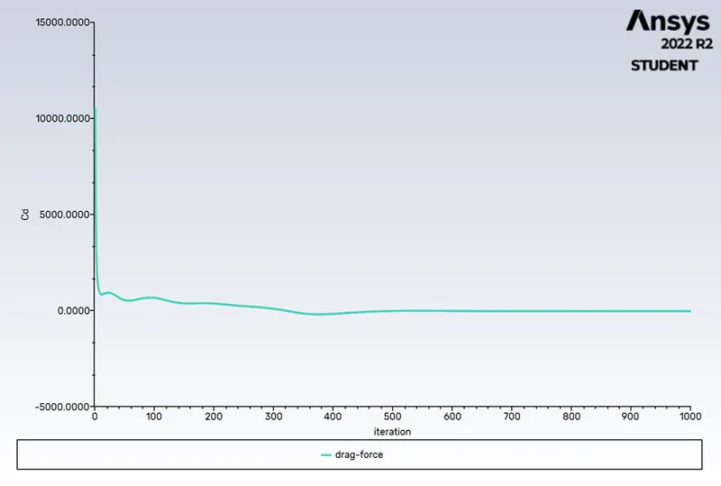
Drag force:

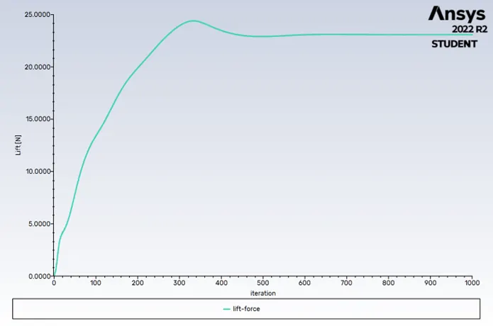
Lift force:

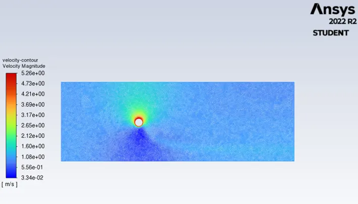
Velocity contour:

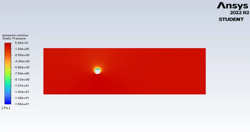
Pressure contour:

Case 2:

Reynolds number: 100

Velocity: 1

Viscosity: 0.02

Iterations: 1000

Residuals plot:

Monitor point velocity:

Drag force:

Lift force:

Velocity contour:

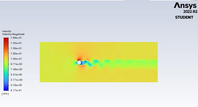
Pressure contour:

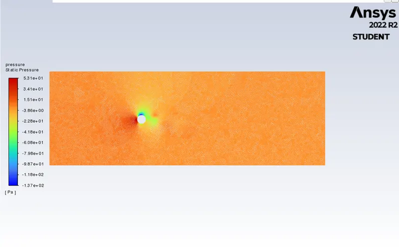
Case3:

Reynolds number: 1000

Velocity: 10

Viscosity:0.02

Iterations: 1000

Residuals plot:

Monitor point velocity:

Drag force:

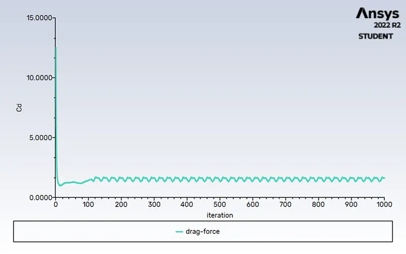
Lift force:

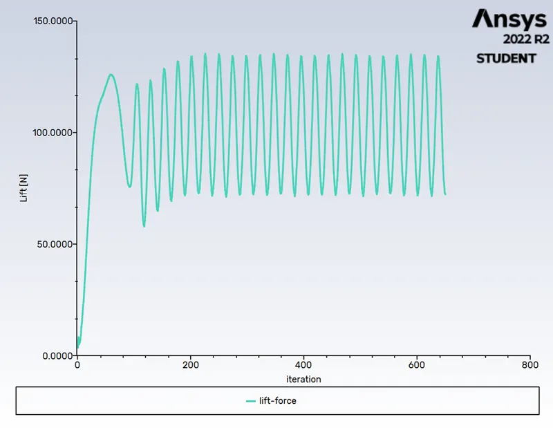
Velocity contour:

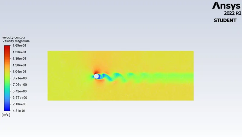
Pressure contour:

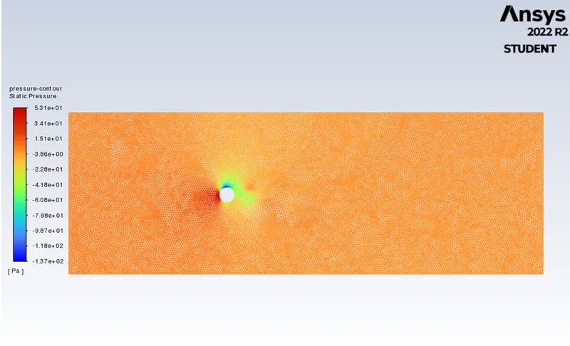
Case 4:

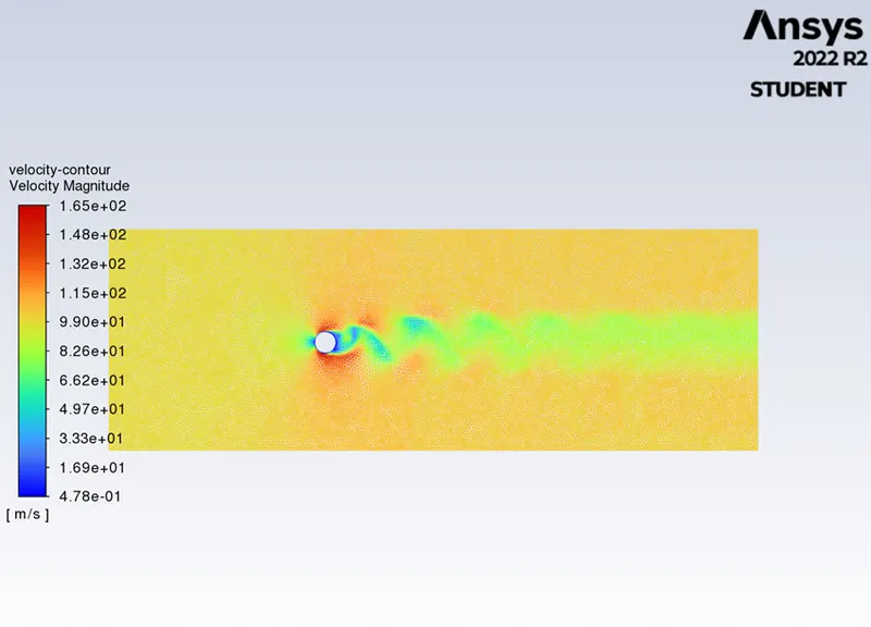
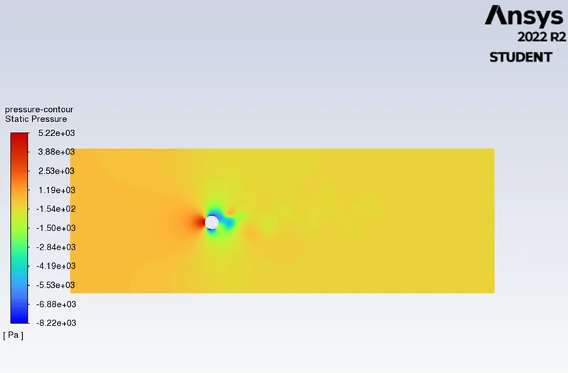
Reynolds number : 10000

Viscosity: 0.02

Velocity:100

Iterations:1000

Residuals plot:

Monitor point velocity:

Drag force:

Lift force:

Velocity contour:

Pressure contour:

Case 5:

Reynolds number: 100000

Viscosity: 0.02

Velocity: 1000

Iterations: 1000

Residuals plot:

Monitor point velocity:

Drag force:

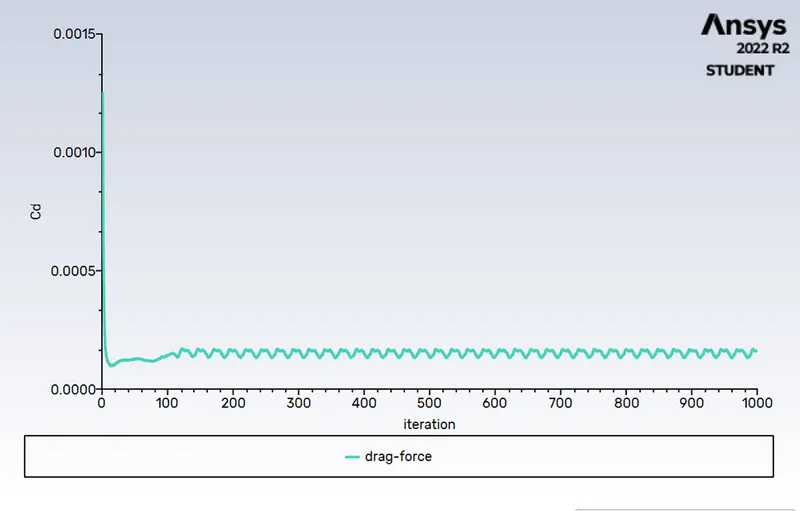
Lift force:

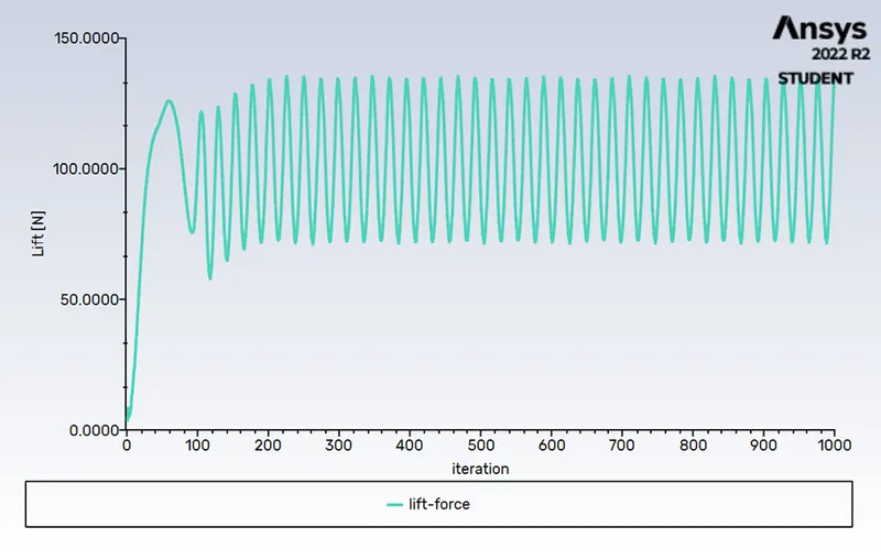
Velocity contour:

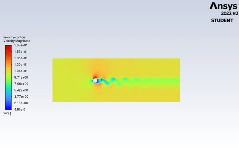
Pressure contour:

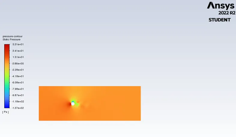
Unsteady state:

Reynolds Number: 100

Viscosity : 0.02

velocity: 1

Iterations : 2000

Time step: 0.2

Residuals plot:

Monitor point:

Drag force:

Lift force:

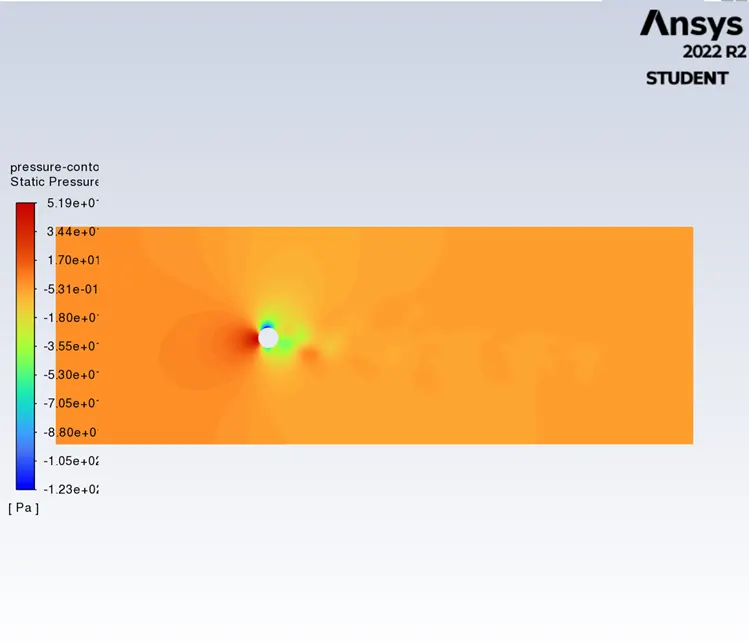
Pressure contour:

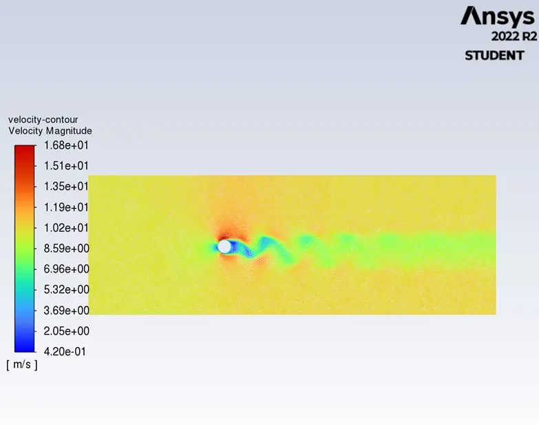
Velocity contour:

Strouhal number:

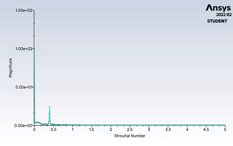
F =number of cycle /time=4/(300-250) =0.08

Strouhal number =(f*l)/v =(0.08*2)/1 =0.16