Week 6 - CHT Analysis on a Graphics card

AIM

• To perform steady state conjugate heat transfer analysis on the model graphics card.
• Run the simulation by varying the inlet velocity from 1 m/s to 5 m/s.
• Find out maximum temperature and heat transfer coefficient attained by processor
• Identify hot spots in the model.

CHT Analysis

The conjugate heat transfer analysis helps to do the simulation of heat transfer between solid and fluid domains by exchanging exchanging thermal energy at the interfaces between them. Applications of this analysis type helps in the design of heat exchangers, cooling of electronic equipment, and general-purpose cooling and heating systems. CHT Simulations help in effieciently designing systems where conductive and convective heat transfer occur and helps reduce the cost and time of development by obtaining an optimized design for testing.

Graphics Card

The wattage of the graphics card is assumed to be 5 W.

Dimensions of the processor : 8mm * 8 mm * 1 mm

Base material : FR-4

Fins : Aluminium

Processor : Silicon

Procedure

• Open the geometry in spaceclaim.
• Make sure the parts of the geometry are under right component name.
• Spaceclaim>workbench>share option to facilitate infromation transfer between shared boundaries and to create a conformal mesh.
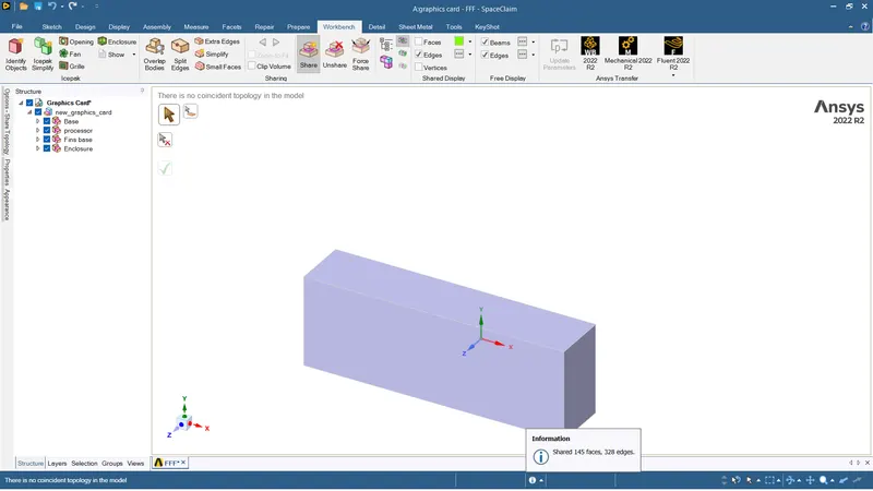
• Close spaceclaim and open the mesh module.
• Generate the default mesh to have a general idea. Make sure the mesh is conformal.

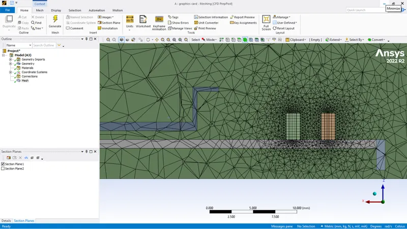
• Refine the mesh using body sizing.

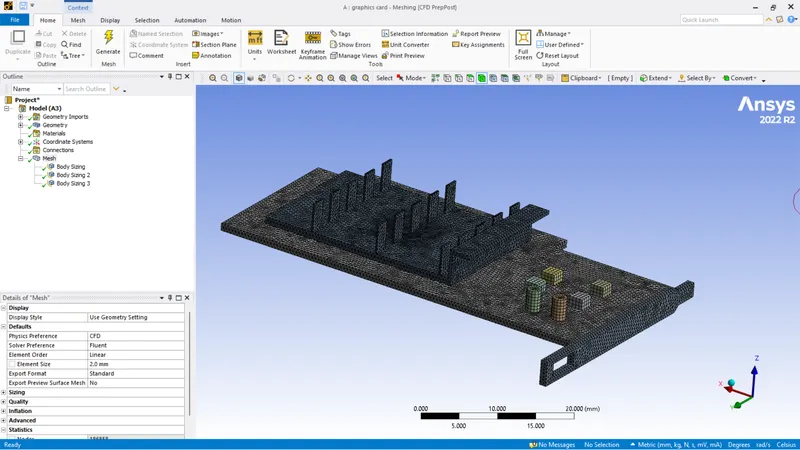
• Once the mesh is refined, we can assign named selections of all the parts of the geometry.
• Close the mesh module and open the setup module with double precision.
• Check mesh for quality.

Type	Pressure Based
Velocity Formulation	Absolute
Time	Steady
Energy	On
Viscous Model	K-Omega SST
Material	Fluid : Air; Solid : Aluminium, FR-4, Silicon
Cell Zones	Defined accordingly as solid materials and air

Fr-4 and silicon was user defined material in solids with the following properties.

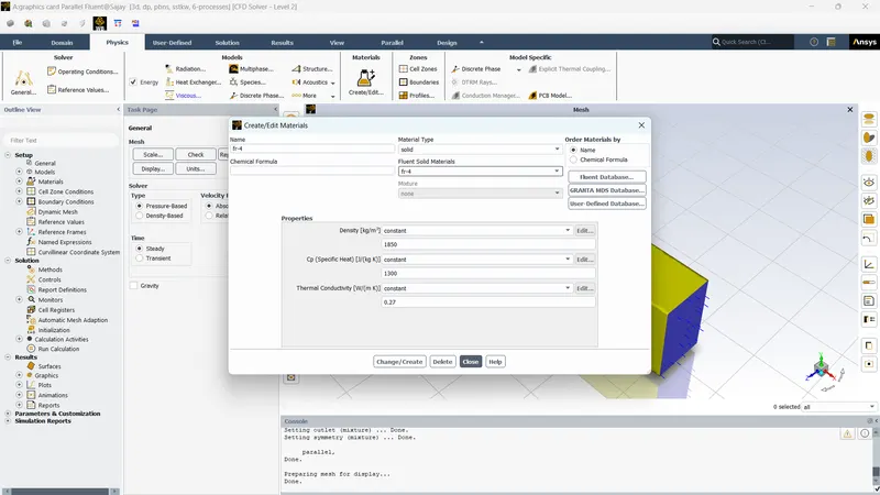
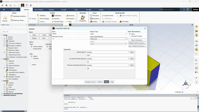
Once the material was defined, we can assign these materials in the cell zones.

Cell Zone for enclosure was assigned as air :

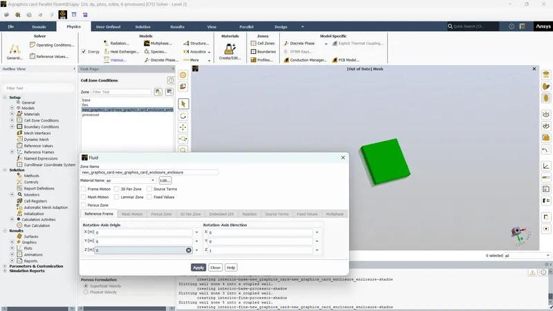
Cell zone for base was assigned as FR-4 :

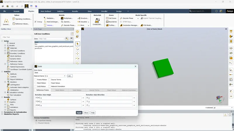
Cell zone for fins was assigned as aluminium :

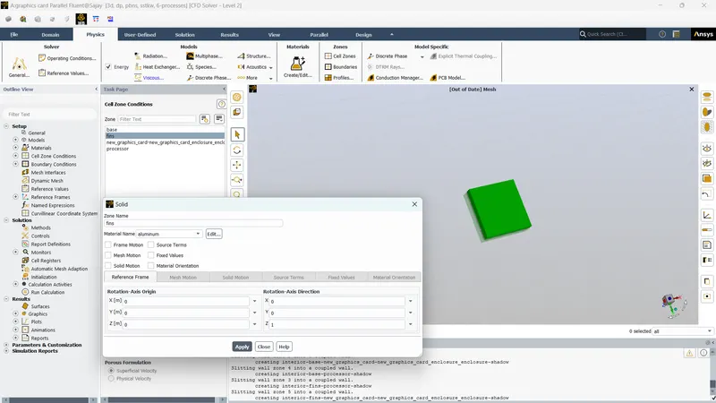
Cell zone for processor was assingnes as silicon with energy source :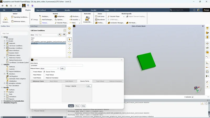

The Power of processor was assumed to be 5 W. Volume of the processor is `64 * 10^-9` `m^3`. Therfore the W/m3 of the energy source is 78125000 W/m3

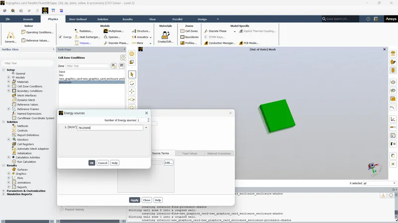
The boundary conditions were assigned as follows:

Inlet	Velocity Inlet; Velocity Magnitude : 1 m/s; Thermal : 300 K
Outlet	Pressure Outlet; Gauge pressure : 0 Pa; Thermal : 300 K
Symmetry	Symmetry
Interior	Interior

Create report definition for heat transfer coefficeint and temperature at the processor.

The solution is initialized using hybrid initialization

Temperature contour of the graphics card and solution animation is created.

The simulation is run for 300 iterations.

Run the same setup for inlet velocity of 3 m/s and 5 m/s.

Results of inlet velocity of 1 m/s

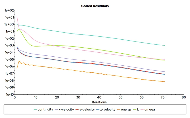
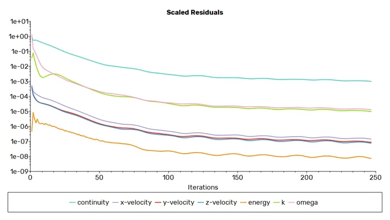
Residuals plot of 1 m/s inlet velocity simulation:

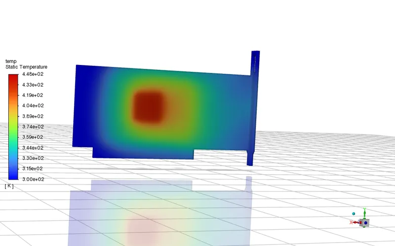
Temperature distribtuion of 1 m/s inlet velocity:

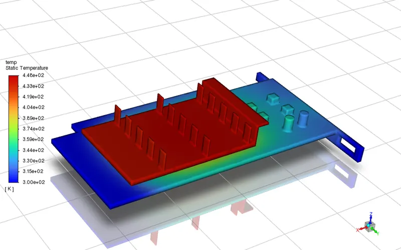
Hotspots with inlet velocity of 1 m/s :

Area-weighted temperature plot of processor :

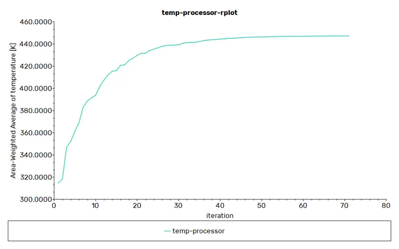
Temperature value at processor :

Area-weighted surface heat transfer coefficient at processor:

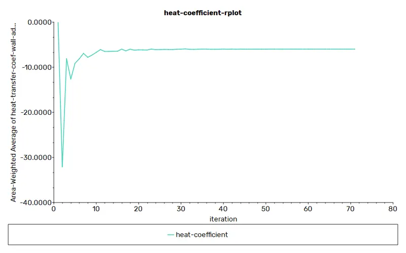
Surface heat transfer coefficient value at processor :

Results of inlet velocity of 3 m/s

Residuals plot of 3 m/s inlet velocity simulation:

Temperature distribtuion of 3 m/s inlet velocity:

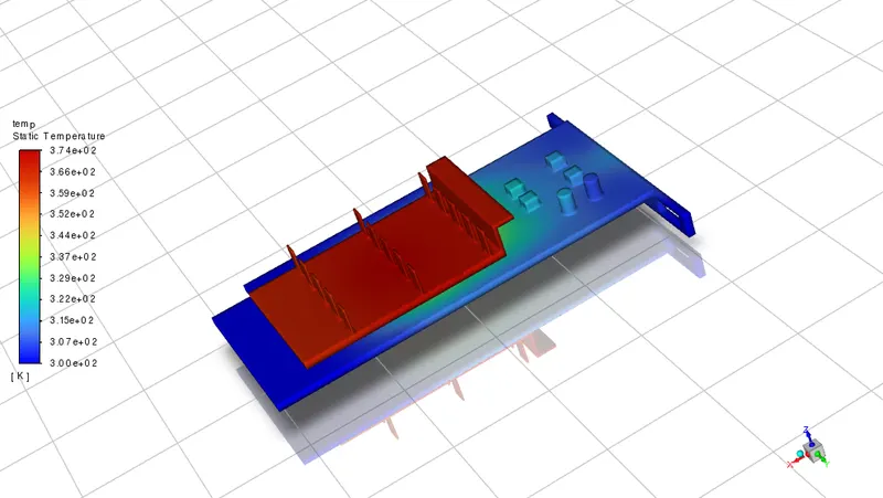
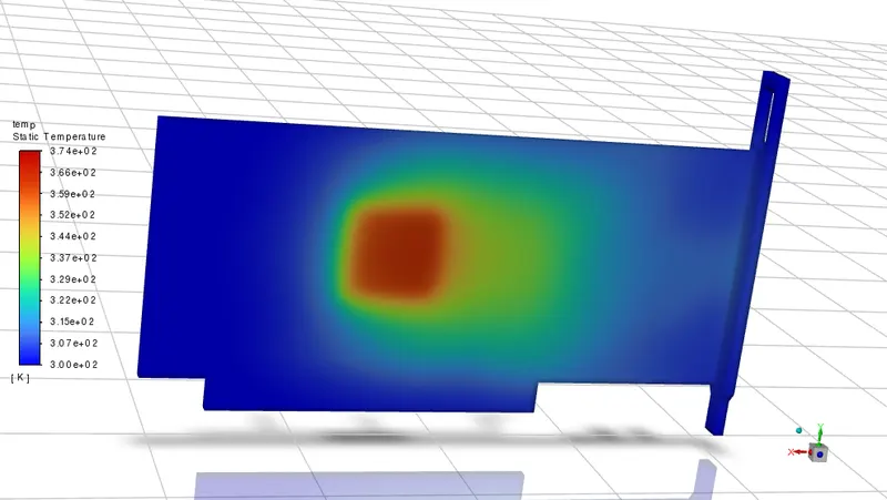
Hotspots with inlet velocity of 3 m/s :

Area-weighted temperature plot at processor :

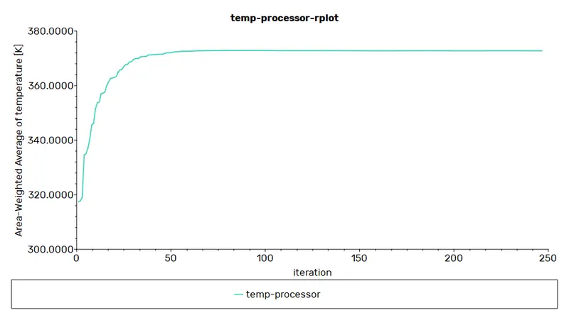
Temperature value at processor :

Area-weighted surface heat transfer coefficient plot at processor :

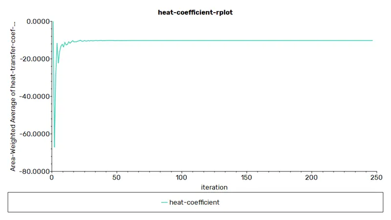
Surface heat transfer coefficient value at processor :

Results of inlet velocity of 5 m/s

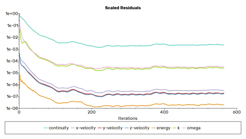
Residuals of inlet velocity of 5 m/s :

Temperature distribution of inlet velocity of 5 m/s :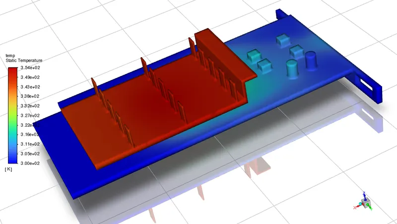

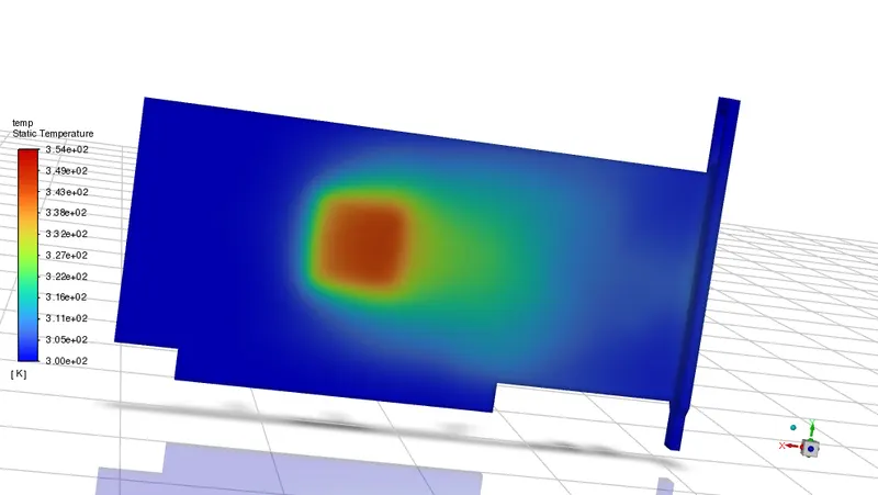
Hotspots of inlet velocity of 5 m/s :

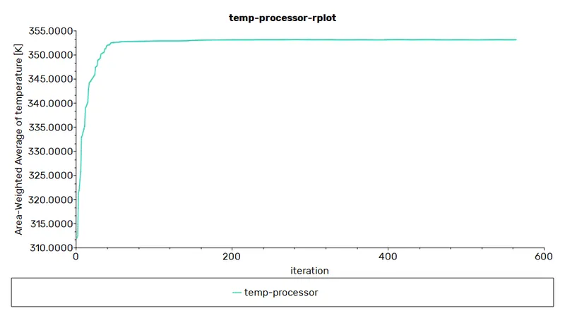
Area-weighted temperature plot at processor :

Temperature value at processor :

Area-weighted surface heat transfer coefficient at processor :

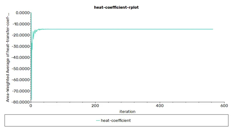
Surface heat transfer coefficient value at processor :

Conclusion

Inlet Velocity (m/s)	Temperature at processor (K)	Surface heat transfer coefficient at processor (W/m2K)
1	447.27	-5.97
3	372.75	-10.23
5	353.15	-14.74

• The residuals plot and report definitions have reached a steady value which shows that the simulation has converged
• Negative sign of heat transfer coefficient indicates that the processor is loosing heat to the surroundings
• The heat transfer coefficient increases with increase in velocity. This inidicates better heat transfer from processor to surroundings.
• The increase in velocity also decreased the processor temperature which is evident from the table
• The hotspot distribution of the 3 cases at the base is shown above. It is evident that increase in velocity decreased the region of hotspots in the base by better flusing of heat to the surroundings.