Week 6 - CHT Analysis on a Graphics card

CHT Analysis on a Graphics card

Aim:To perform a steady-state conjugate heat transfer analysis on a model of a graphics card.

Objectives:

1. To run the simulation by varying the velocity from 1m/sec to 5m/sec for at least 3 velocities and discuss the results.
2. To find out the maximum temperature and heat transfer coefficient attained by the processor.
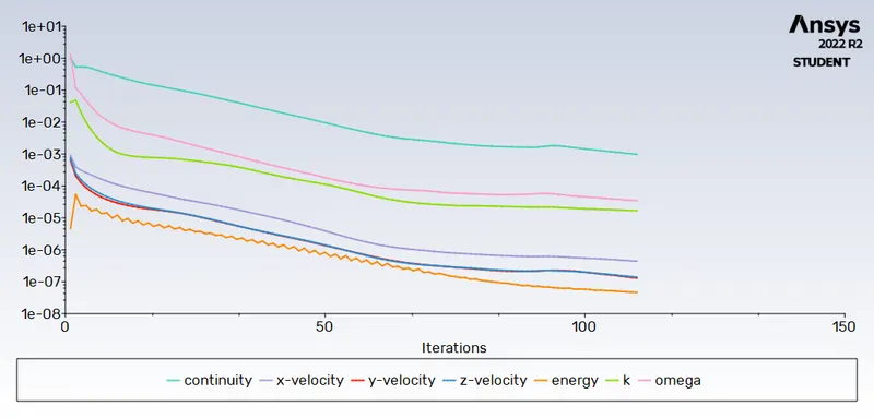
3. To prove that the simulation has achieved convergence with appropriate images and plots.
4. To identify potential hotspots on the model.

Introduction and Theory:

CHT analysis and its applications:

The Conjugate Heat Transfer (CHT) analysis allows for the simulation of heat transfer between solid and fluid domains by exchanging thermal energy at the interfaces between them. Typical applications of this analysis type exist as, but are not limited to, the simulation of heat exchangers, cooling of electronic equipment, and general-purpose cooling and heating systems.

Examples:

HVAC, Heat Exchanger, Tank, Internal Combustion Engine, Heat Sink, Boiler, Reactor, Heat Pipe, Turbocharger.

The CHT approach has an advantage over FE thermal analysis in that wall heat transfer coefficients and their local variations on surfaces are directly calculated within the model rather than based on simplified empirical calculations. The CHT approach therefore has benefits for those applications where heat transfer is either non-uniform or difficult to calculate empirically.

Solving and Modelling :

Geometry creation:

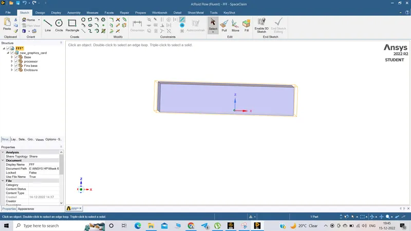
Importing geometry in spaceclaim and share topology to reduce the interferences.

Meshing:

Meshing with combination of coarse and refined mesh in different regions:

Named selection and by inserting method :

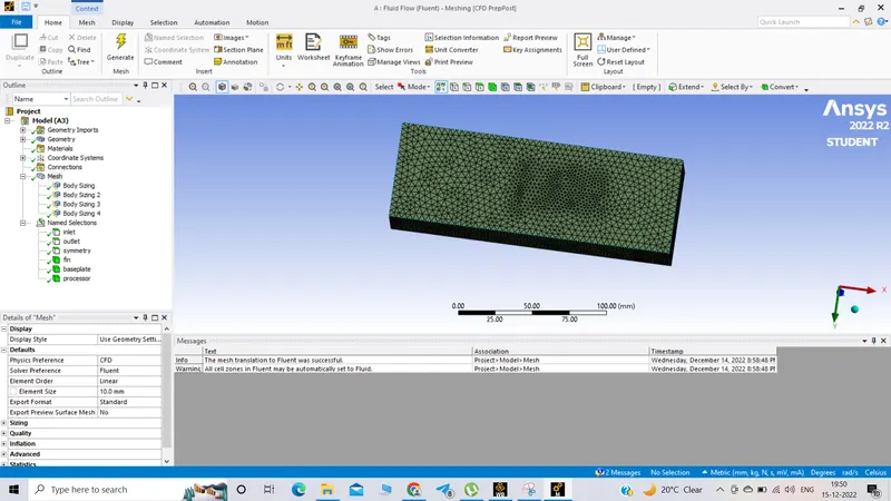
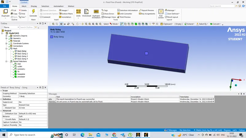
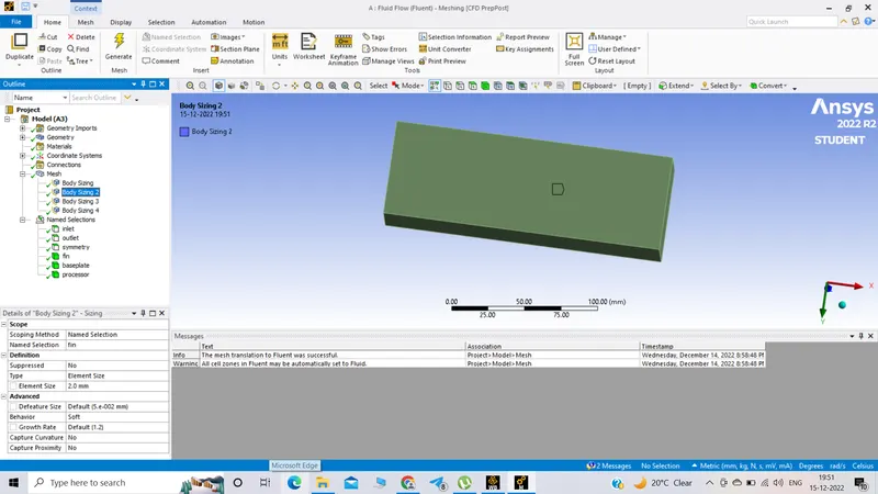
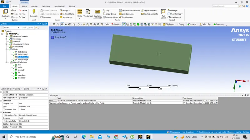
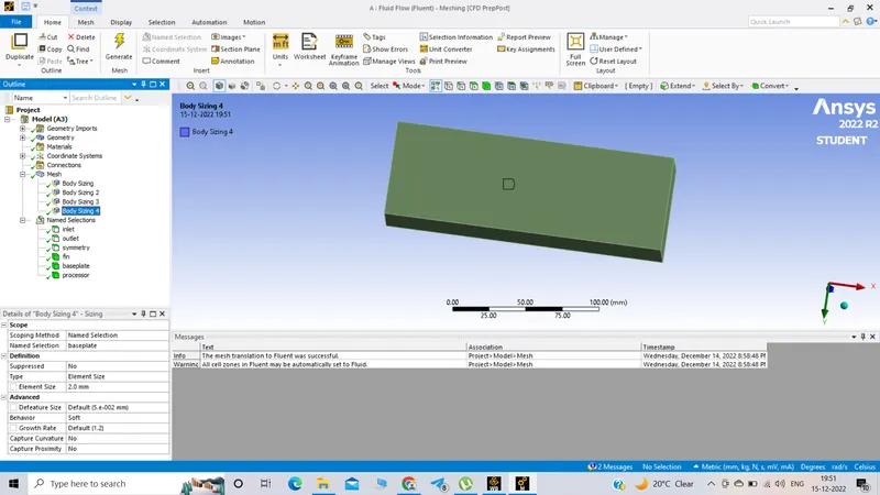
The reason for choosing the particular mesh setting is to find an accurate result.

Setup:

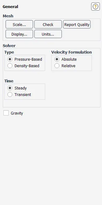
General setup:Energy equation is enabled.

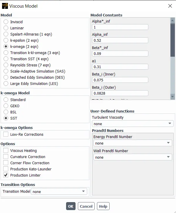
Viscous Model:

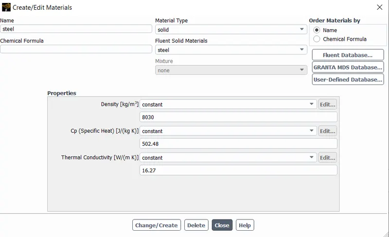
Materials:

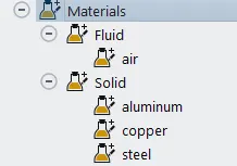
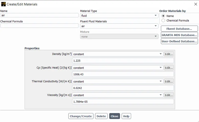
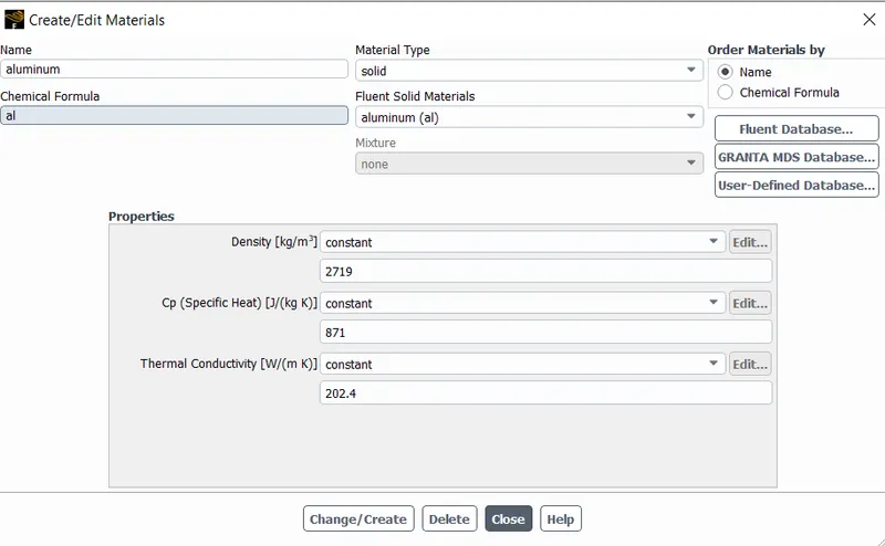
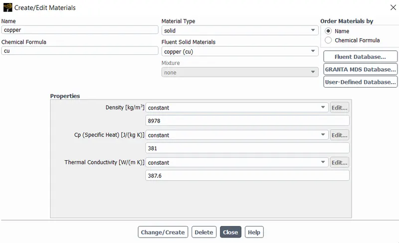
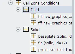
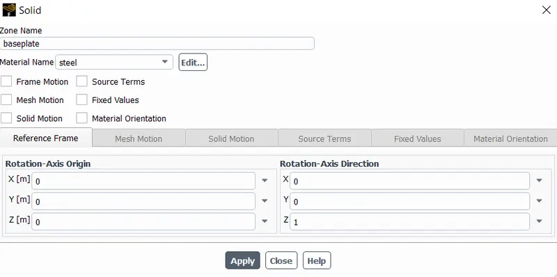
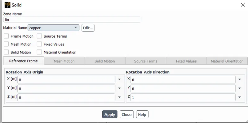
Cellzones:

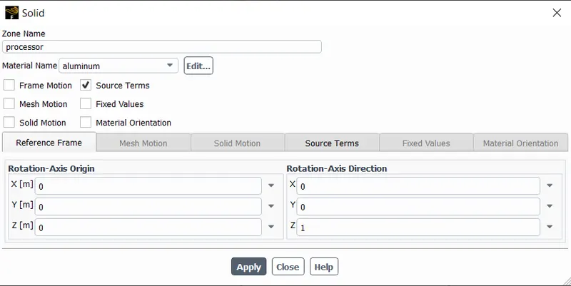
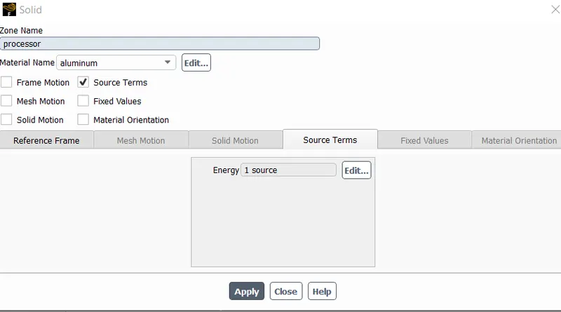
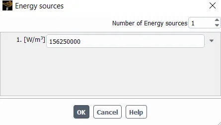
The heat should be applied to the processor as Energy Sources (Source term) by considering the heat produced and volume of the processor.

Graphics Card Power = P=10W

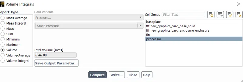
Volume of the processor=V=6.4e-08 `m^3`

Energy produced by the processor=P/V=156250000 `W/m^3`

Boundary condition:

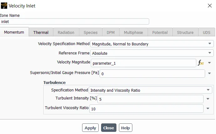
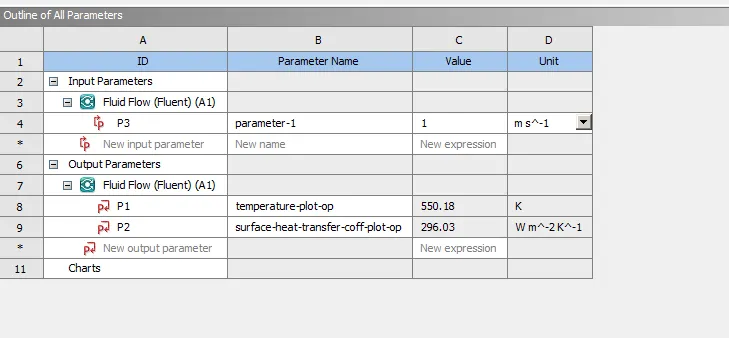
Velocity input is given parametric (1m/sec , 3m/sec,5m/sec)

Solutions:

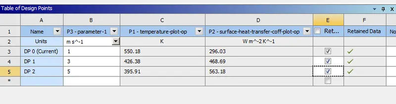
Parametric :

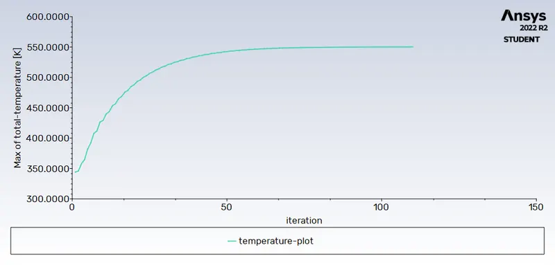
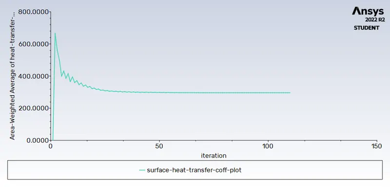
For velocity 1m/s

Residuals:

Temperature plot:

Surface heat transfer coefficient plot:

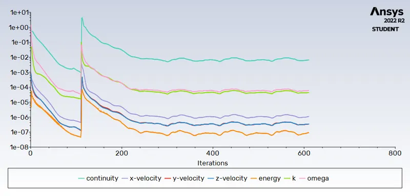
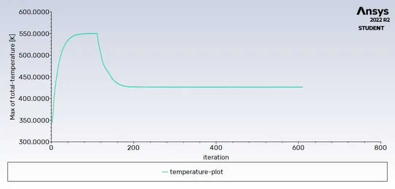
For velocity 3m/s

Residuals:

Temperature plot:

Surface heat transfer coefficient plot:

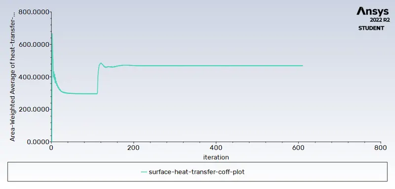
For velocity 5m/s

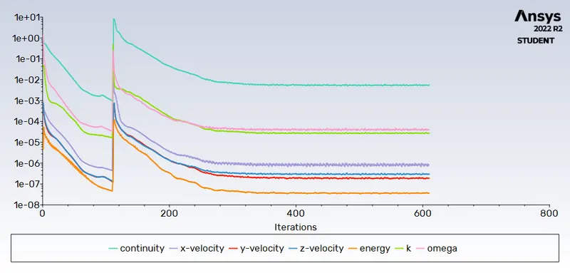
Residuals:

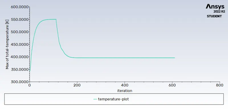
Temperature plot:

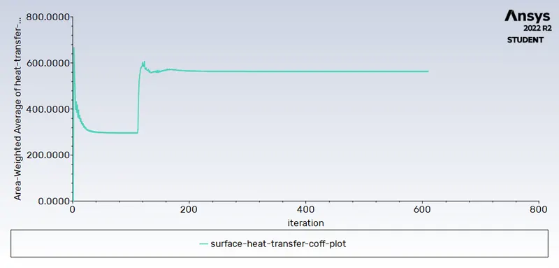
Surface heat transfer coefficient plot:

Result:

For velocity 5m/s

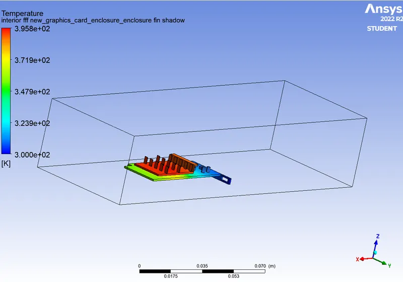
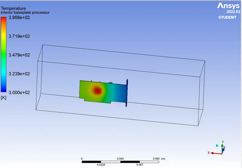
Temperature plots:

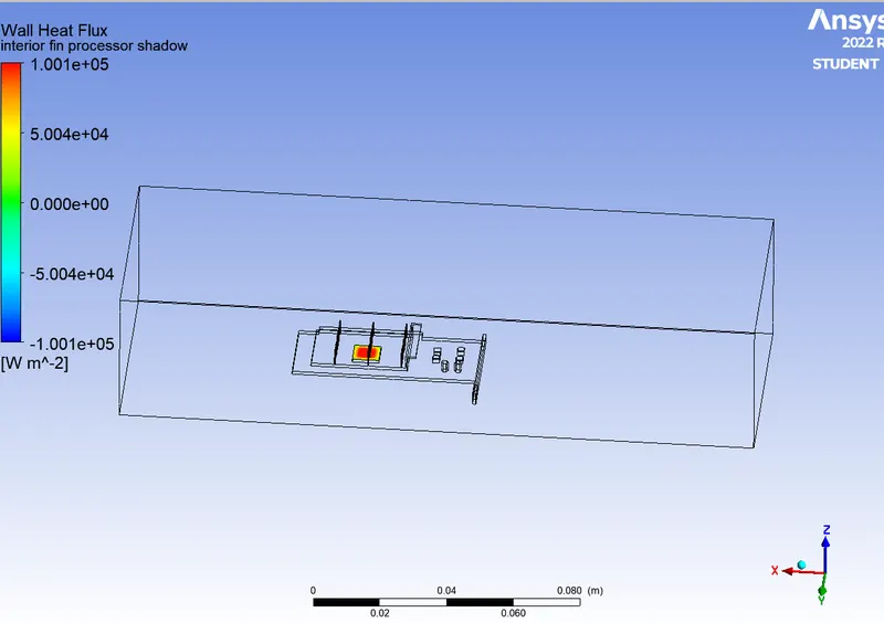
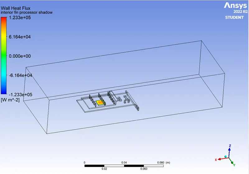
Wall heat flux plot:

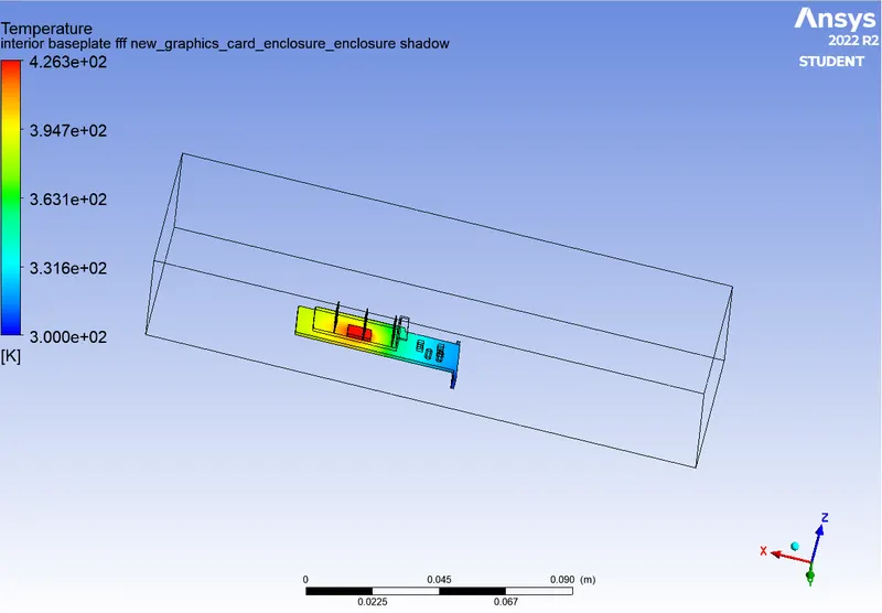
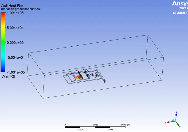
For velocity 3m/s

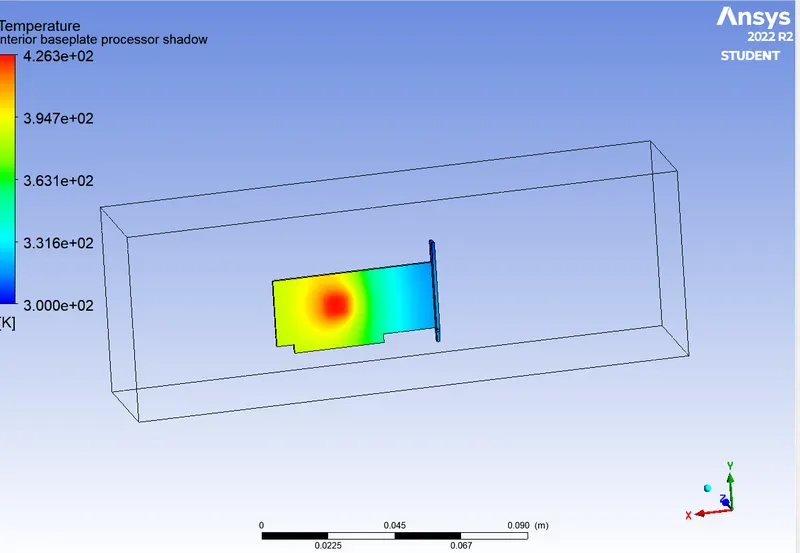
Temperature plots:

wall heat flux:

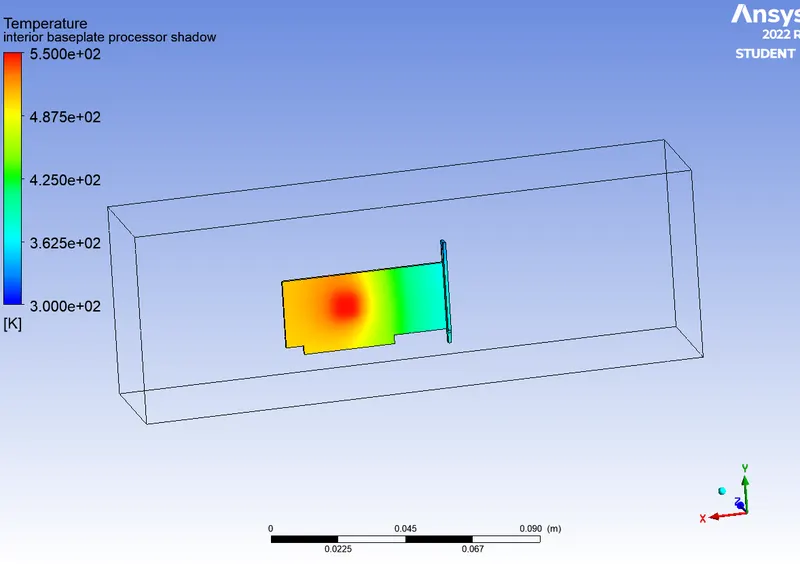
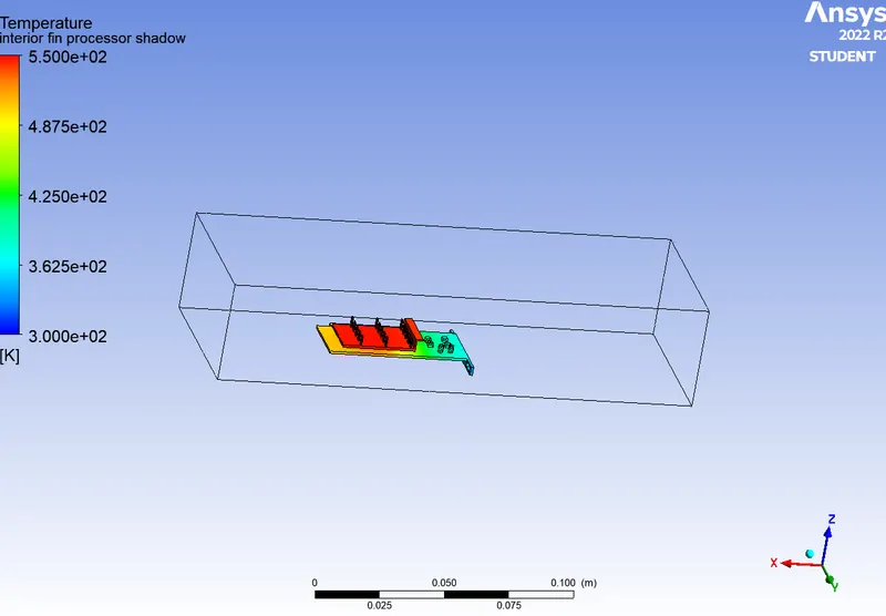
For velocity 1m/s

Temperature plots:

wall heat flux:

A converged solution for the given sets of input was observed on the basis of repetitive plots in the Residual plot. The processor acted as a source of heat input .With an increase in velocity, we saw a considerable drop in temperature and a substantial rise in heat transfer coefficient which shows that high-velocity air can be an effective mode of heat dissipation in graphics card.

The high-temperature regions are found at the center of the fins, base, and the processor walls. From the temperature distribution, we can see hotspots in the fin and base near the surface that is in contact with the processor. Based on the thermal conductivity of the material this temperature is distributed accordingly amongst the component. We see a few high-temperature zones on fin away from processor depicting their high susceptibility to heat due to their geometry.

Conclusion:Conduction occurs where there is a contact region between the solids in this case it is between processor ,fins and and base. Convection occurs when the heat generated in the components of the graphic card is removed by the inlet airflow.