Week 6 - CHT Analysis on a Graphics card

AIM -

A steady-state simulation for Conjugate Heat Transfer (CHT) analysis of Graphics Card to be performed using Ansys Fluent.

INTRODUCTION -

Conjugate Heat Transfer (CHT) is the exchange of thermal energy at the interfaces of solid and fluid domains to transfer heat. That is, it includes both conduction and convection heat transfer modes. Conjugate Heat Transfer is demonstrated by heat exchangers, electronic device cooling, and cooling and heating systems.

Graphics Card -

A graphics card is a piece of hardware that boosts a computer's video memory and improves the display quality. It increases the computer's power and enables it to perform more demanding tasks. The graphics card's quality affects the image's quality.
Rendering graphics is the main function of graphics cards. Your computer cannot display any information or perform as you need it to without a graphics card. To put it simply, the GPU uses information from the processor and software to decide where to place pixels on the screen.

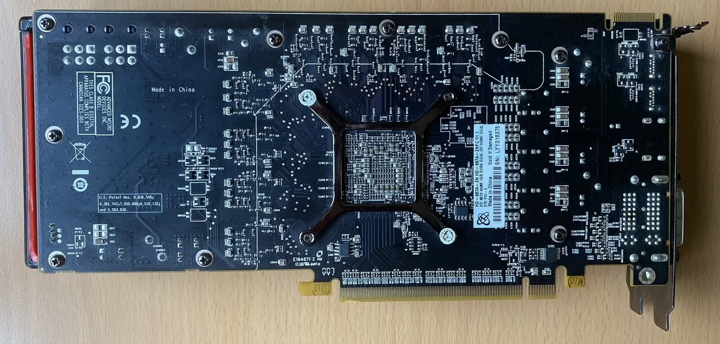The provided model of a graphics card comprises of processor, fins, board, and an enclosure to cover the entire assembly. This enclosure will act as the computational domain to perform the desired numerical simulation.

In this geometry of the graphics card model, the conjugate heat transfer takes place as;

• Convection takes place between the fluid (air) and the processor
• Conduction takes place between the processor and the fins
• Convection takes place between the fins and the surrounding

The use of fins with processors is intended to increase the processor's surface area so that more heat transfer occurs due to an increase in the rate of heat dissipation and one can use the graphics card or the associated device at its best performance levels.

THEORY -

Extended Surfaces - Fins

Fins are extended surfaces attached to the primary objects to be cooled. For example, motorcycle cylinder heads & finned tubes in heat exchangers. Fins are a conduction-convection system employed to dissipate heat from a surface at a faster rate to the surrounding fluid. Heat conducts from the primary object into the fins. The fin surface provides an extra surface for heat dissipation to take place via a convention. In a nutshell, it can be said that fins are used to enhance the heat transfer process.

Fin Effectiveness:

It is a measure of how much heat is conducted by fins compared to heat conducted from the base area without the fin.

`eta_(effect) = frac{Q_(with Fi n)}{Q_(w//o Fi n)}`

Fin effectiveness is improved by using a material with large thermal conductivity. The effectiveness of a fin can be improved by improving the 'P/A' ratio (Perimeter/Area).

Fin Efficiency:

It is a measure of heat transferred by the fin to the heat transferred by an ideal fin of the same geometry. The ideal fin is the one that is kept at the base temperature throughout the length.

`eta = frac{q_(fi n)}{q_(ideal fi n}`

High efficiency is not always a major of the high-performing fin. Effectiveness must also be considered.

SOLVER & MODELLING APPROACH -

The following is the workflow with each CFD simulation:

1) Problem finding
2) Pre-processing
3) Processor or Solver
4) Post-processing

The properties of any material that must be assigned for any heat transfer analysis problem are its density(`rho`), specific heat capacity(`cp`), and thermal conductivity (`k`).

In this CHT simulation, we assigned the board a polystyrene material as the board should possess good insulation characteristics. The fins body was assigned with aluminum material and the processor was assigned with silicon.

Essential properties for the above-assigned materials will be taken as:

Material	Density (`rho`) [kg/m³]	Specific Heat Capacity (`cp`) [J/kg K]	Thermal Conductivity (`k`) [W/m⋅K]
Silicon (Processor)	2330	703	153
Polystyrene (Board)	55	1210	0.027
Aluminium (Fins)	2719	871	202

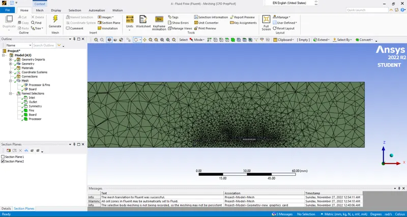
The "Share" tool was used during the pre-processing to share the topology between the coincident surfaces after importing the geometry model of the graphics card into SpaceClaim. The components of the graphics card were given names using the 'Named Selection' command and mesh generation over geometry was done in the mesh file. In the setup file, the simulation was run with the appropriate solver settings, and as post-processing, results were calculated in the form of contours in the result file. After analyzing the outcomes, conclusions were met.

Here, simulations with varying inlet velocities of 1 m/s, 3 m/s, and 5 m/s were run with a coarse mesh in accordance with the problem statement. A refined mesh was later created for additional one or two cases as part of a mesh-independent study, and results from these simulations were obtained. As a result, simulations for five cases were run.


PRE-PROCESSING -

In SpaceClaim, import the geometry model of the graphics card and use the 'Share' tool under the 'Workbench' toolbar so that the coincident faces (or surfaces) share the mesh information.

In the 'Mesh' file, using the 'Name Selection' command, assign the components of the graphics card with relevant names as:

1. Inlet (the inlet of the enclosure)
2. Outlet (the outlet of the enclosure)
3. Symmetry (four walls of the enclosure)
4. Processor
5. Fins
6. Board

Element size and cell counts employed during mesh generation were as:

Mesh Type	Case No.	Element Size (mm)			Cell Count (lacs)
		Base Mesh	Processor & Fin	Board
Coarse	1, 2 & 3	8	1	1	1.48
Refined	4	7	0.75	0.75	3.34
Refined	5	6	0.6	0.6	4.96

SOLVER -

Before proceeding with the solver settings, it is necessary to find out the heat generation rate of the processor so that it could be assigned to the processor as the source of energy in the 'Cell Zone' condition.

The volume of the processor `(V)` was found to be `8 mm xx 8 mm xx 1 mm = 64 mm³`. As the volume of the processor is very small, the considered value of the heat dissipation rate of the processor `(q)` was 1 watt.

Thus, heat generation rate of processor `= frac{q}{V} = frac{1}{(64xx10^-9)} = 15625000 frac{W}{m³}`

In the Setup file, provide the following solver settings:

Fluent Setup
Sr. No.	Setup	Command
1	Solver Type	Pressure based
2	Solver Time	Steady State
3	Energy	ON
4	Turbulence Model	K omega SST
5	Materials	Fluid - Air
		Solid - Aluminium (Fins), Silicon (Processor) & Polystyrene (Board)
6	Inlet	Velocity Inlet – 1 m/s, 3 m/s & 5 m/s
7	Outlet	Pressure Outlet
8	Method	Coupled

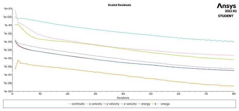
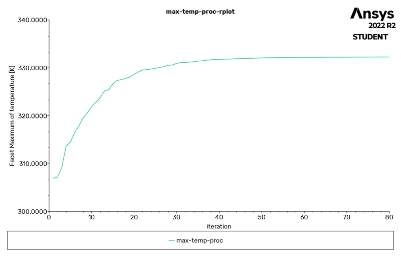
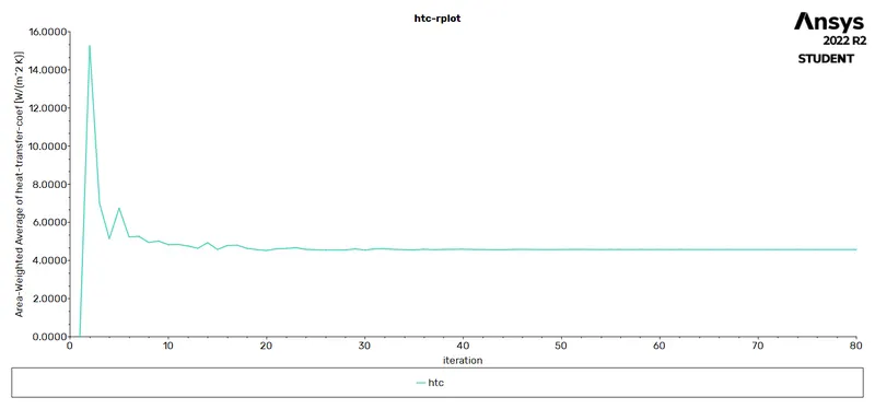
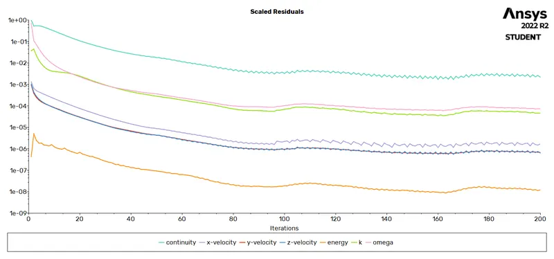
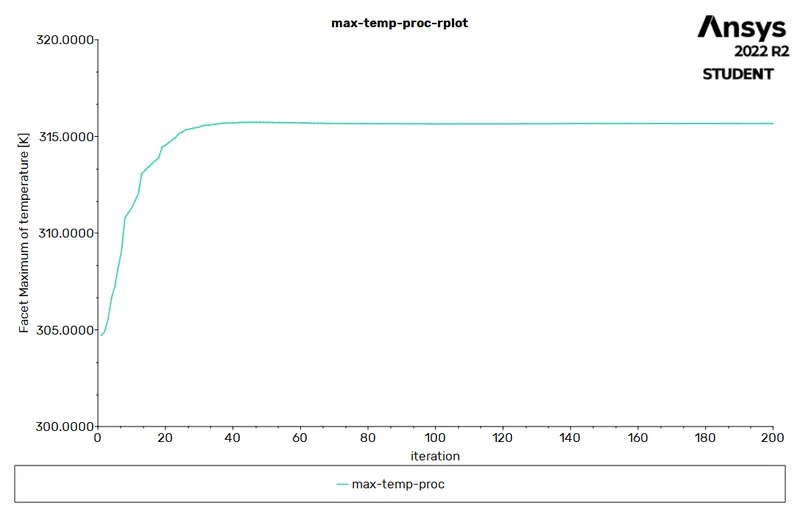
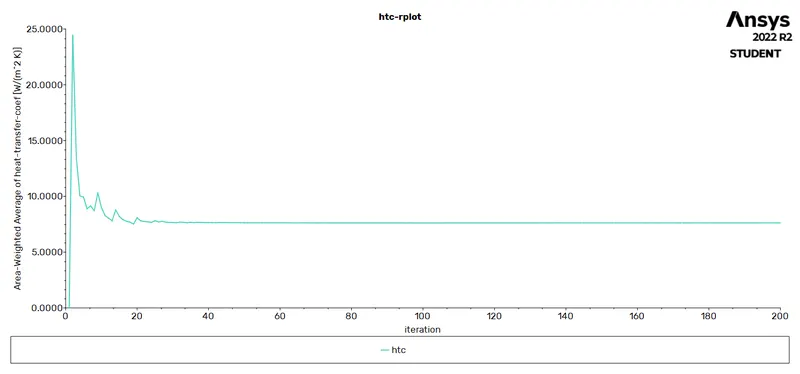
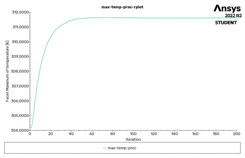
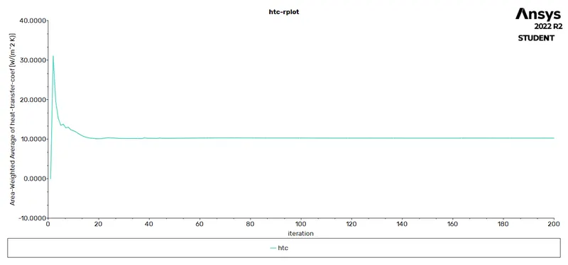
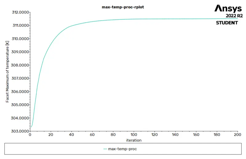
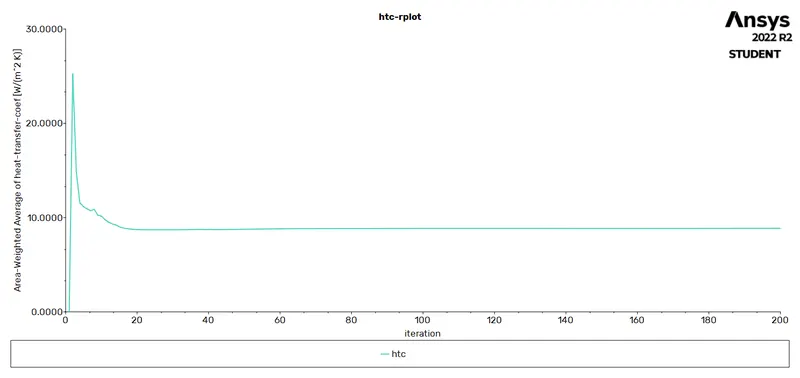
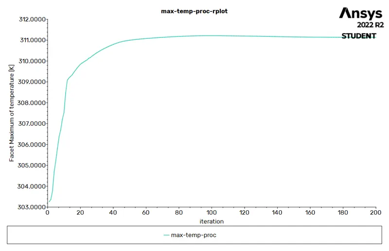
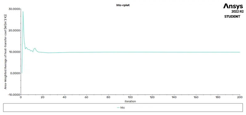
As we need to find the maximum temperature and the heat transfer coefficient of the processor, A report to calculate the maximum temperature and the heat transfer coefficient of the processor was prepared using the 'Report Definitions' tool.

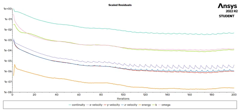
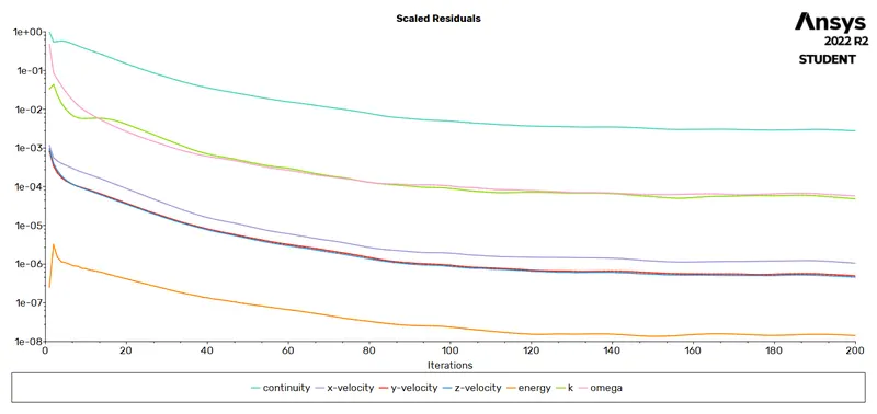
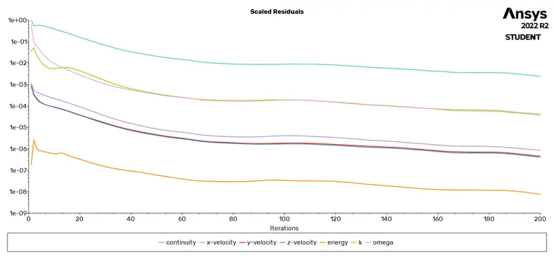
Initialize the solver settings and ran the simulation, for all five cases, for a certain number of iterations till convergence was achieved.

Case No.	Plots
	Scaled Residuals	Maximum Temperature	Heat Transfer Coefficient
1
2
3
4
5

POST-PROCESSING -

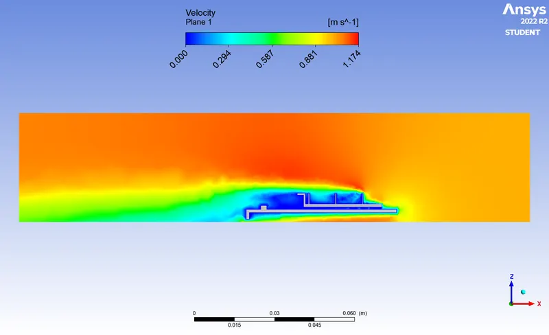
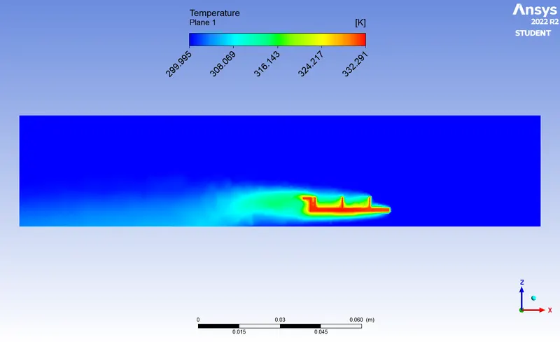
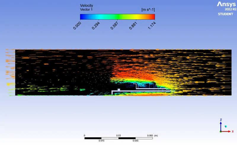
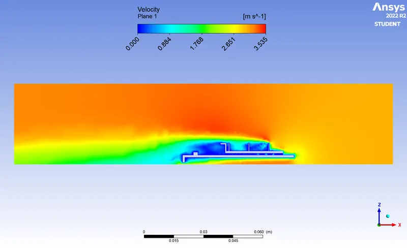
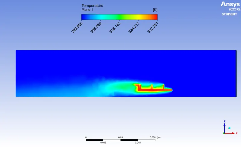
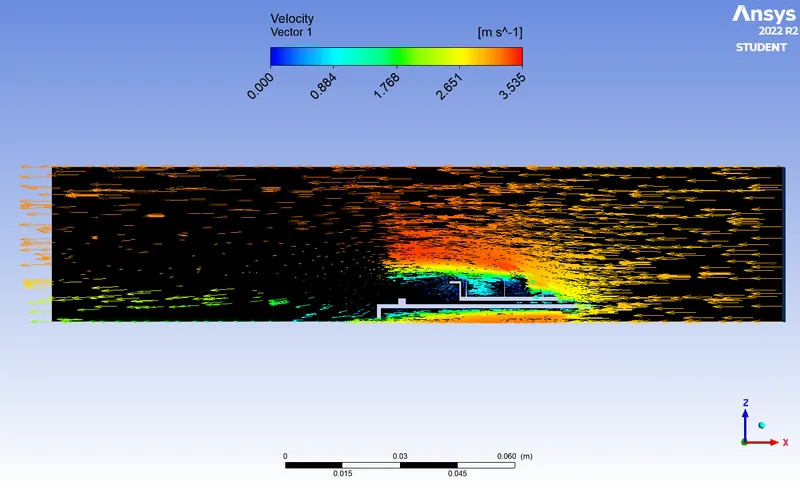
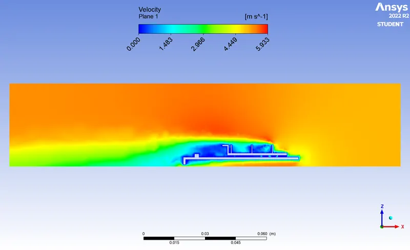
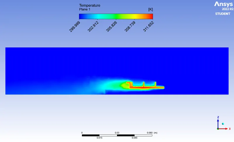
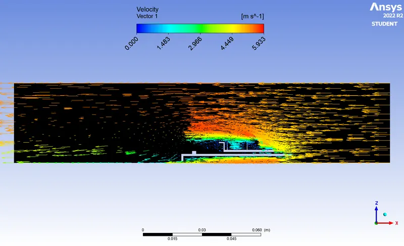
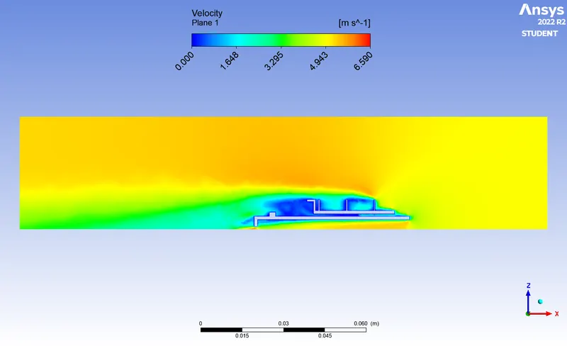
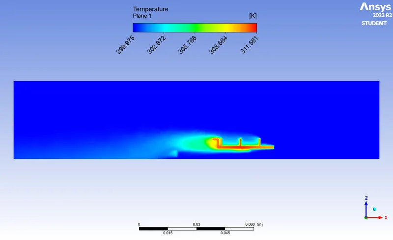
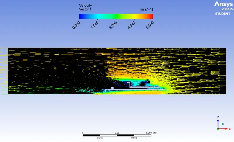
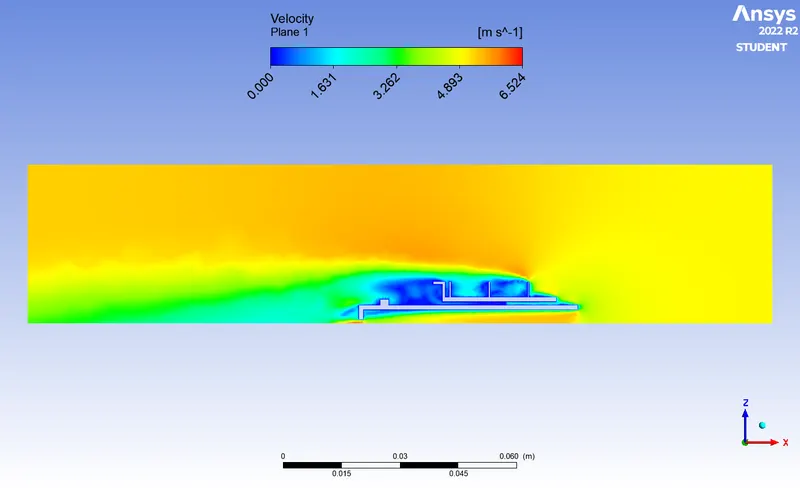
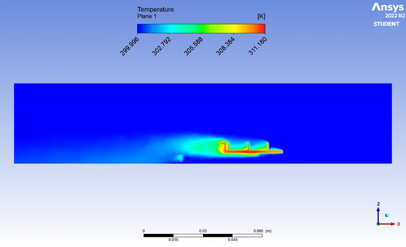
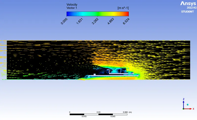
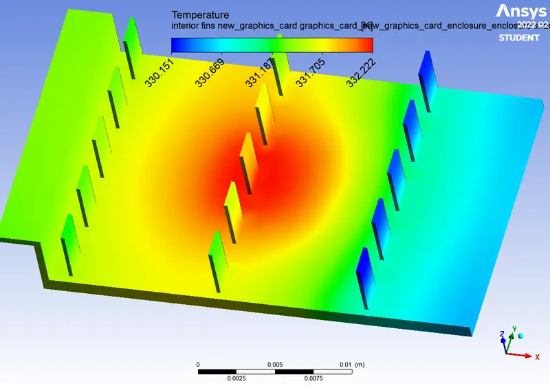
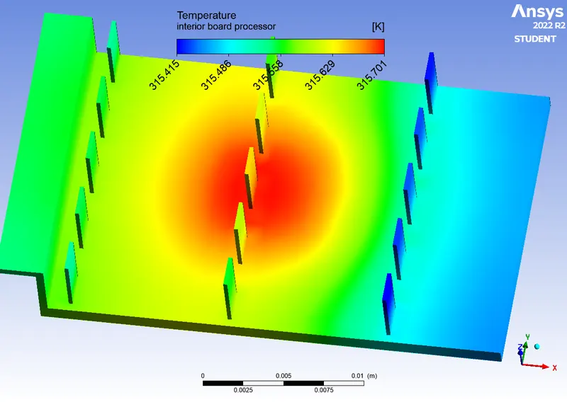
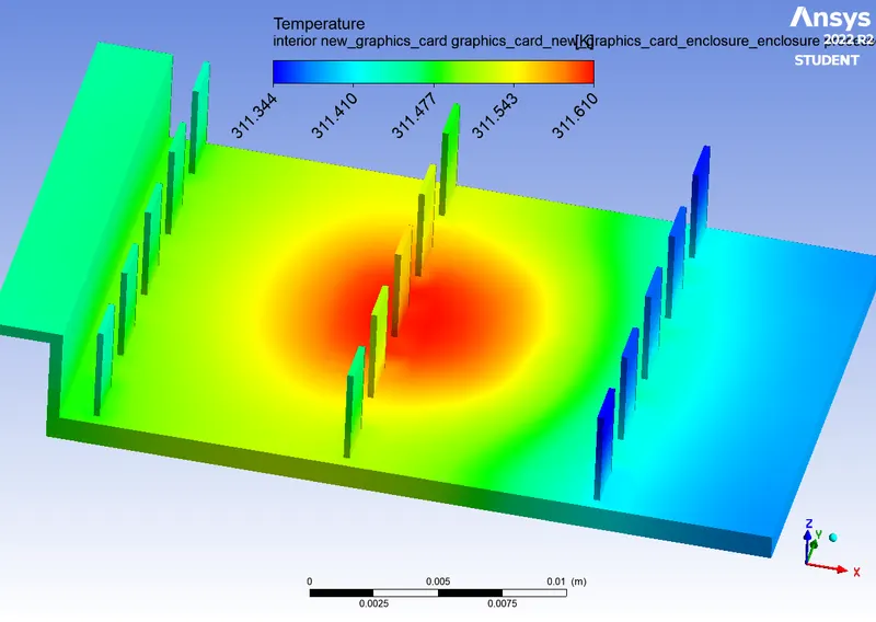
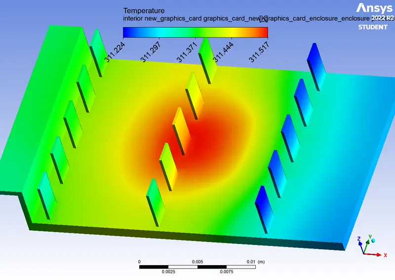
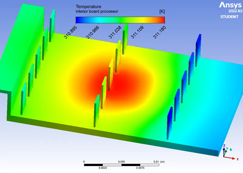
Contours for velocity, temperature, and velocity vector over a plane parallel to the fluid flow were plotted and saved. Also, the potential hotspots were identified on the graphics card model.

RESULTS -

Case No.	Contours
	Velocity	Maximum Temperature	Velocity Vector
1
2
3
4
5

Case No.	Potential Hotspots
1
2
3
4
5

CONCLUSION -

Case No.	Mesh Type	Cell Count (lacs)	Velocity (Inlet) [m/sec]	Maximum Temperature [K]	Heat Transfer Coefficient [W/m2K]
1	Coarse	1.48	1	332	4.6
2	Coarse	1.48	3	315	7.6
3	Coarse	1.48	5	311	10.3
4	Refined	3.34	5	311	8.9
5	Refined	4.96	5	311	9.9

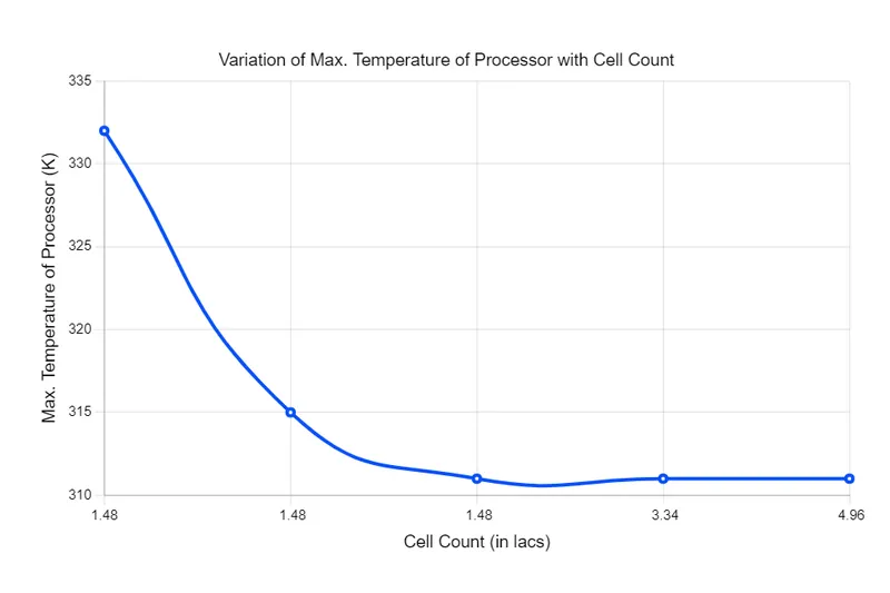
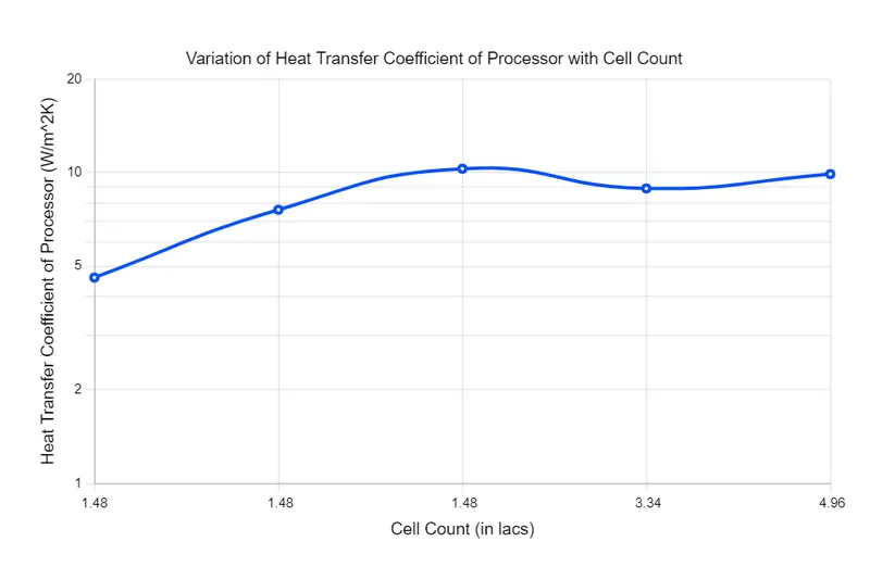
A few conclusions about the study of CHT analysis over the graphics card can be drawn after operating the simulation for all five cases;

1. The temperature of the processor continues to drop as the velocity input at the inlet rises. At a certain velocity limit, however, no such tendency in temperature decrease is seen.
2. With an increase in velocity at the inlet, a somewhat similar trend is seen in the heat transfer coefficient value increment. However, this increment converges at a certain point and stops increasing altogether.
3. The heat transfer coefficient is highest and the processor's maximum temperature is lowest when the inlet velocity is 5 m/s. This results in a higher rate of heat dissipation. Therefore, it can be inferred that for this problem statement, the case with an inlet velocity of 5 m/s is preferable for the processor than the other cases.
4. According to this CHT analysis study, potential hotspots are the high-temperature regions observed at the processor and the fins. As the processor generates heat and dissipates it to its surroundings, we can see a potential hotspot in this region. As the magnitude of the inlet velocity increases, the temperature at the hotspot region decreases, which is satisfactory for the graphics card.

Thus, the study of simulation for Conjugate Heat Transfer (CHT) analysis over a Graphics Card was accomplished using Ansys Fluent.