Week 6 - CHT Analysis on a Graphics card
Aim/Objectives
To perform steady-state conjugate heat transfer analysis on a model of a graphics card.
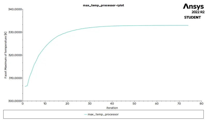
To find the maximum temperature and heat transfer coefficient attained by the processor.
Conjugate Heat Transfer (CHT)
Conjugate Heat Transfer (CHT) is a analysis of heat transfer between a solid and fluid domain by exchanging the thermal energy at the interface between them.
CHT analysis are used in many engineering applications wherever there is a heat transfer between solid and fluid domain such as HVAC, electronic component design, cooling system design, heat exchangers, battery thermal management and exhaust manifold.
Pre-processing
Geometry
Initially the geometry is imported into the spaceclaim using ansys workbench.
After importing geometry share topology is enabled to share its topology with its neighbouring faces.
Geometry consist of four parts such as :
PCB Board - Acts as an support for the processor and other electronic components.
Processor - Heat generating component.
Fins - Consist of extended surface for heat dissipation.
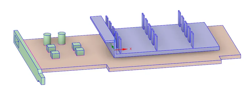
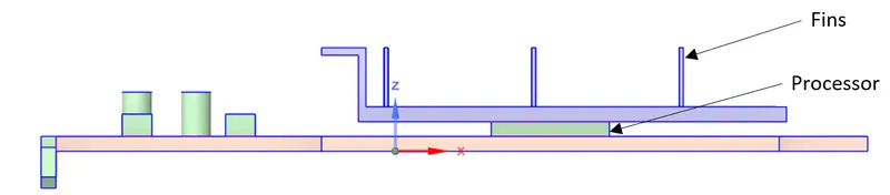
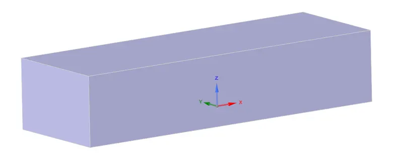
Enclosure - Fluid domain for simulation.
Mesh
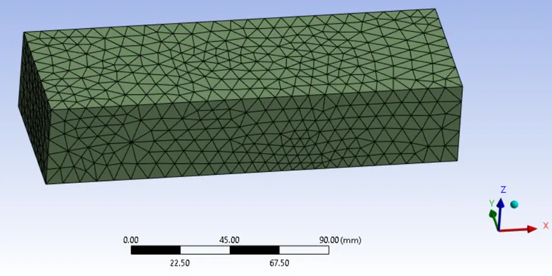
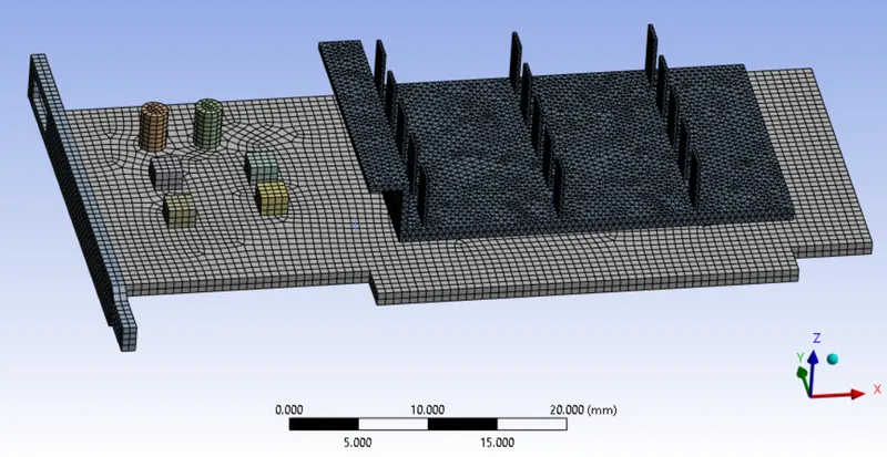
Mesh generation is performed for two cases one for coarse mesh and another one with finer mesh.
Coarse mesh has an total mesh elements of 238232.
Fine mesh has an total mesh elements of 456345.
While meshing it is ensured that it has formed a conformal mesh so that the mismatch of mesh elements could be achieved and solution is accurate.
Solver settings
Setting up physics
Steady state pressure based solved is used.
Energy is turned on as temperature is involved in this case.
Viscous model is set to K-omega SST model.
Material properties used for this simulation is given below:
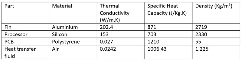
In cell zones the material type for the fins, processor and PCB is set to solid and appropriate material is selected.
Heat dissipation rate of processor is assumed to be one watts. More the watts more the heat generation will be.
Hence heat generation of processor is assumed as 15625000 W/m3
Boundary conditions for the inlet is velocity inlet. Here the velocity is varied inbetween 1 to 5 m/s.
Setting up the solution
The hybrid initialization is initialized.
Temperature and heat transfer coefficient are set to be identified.
Results
Case : 1 For fluid flow velocity of 1 m/s
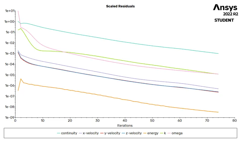
Residulas
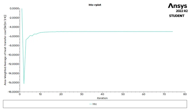
Heat Transfer Coefficient
Maximum Temerature of The Processor
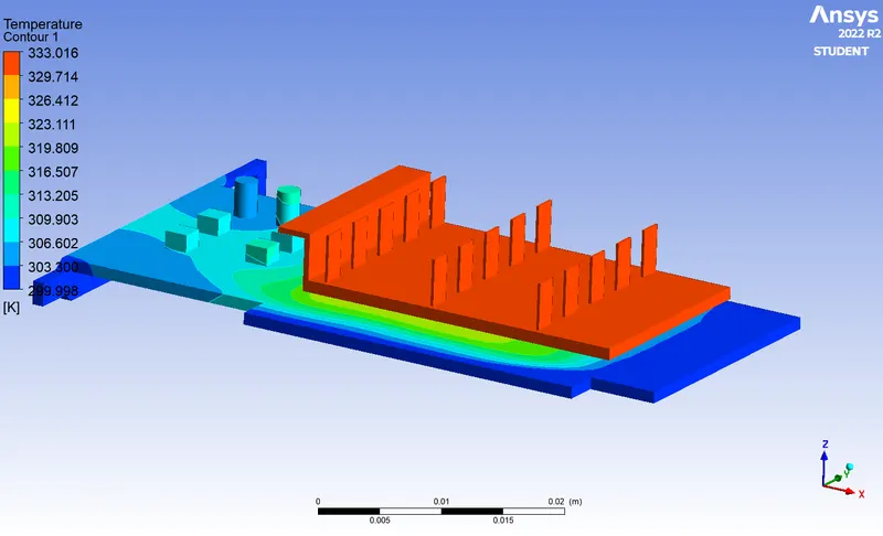
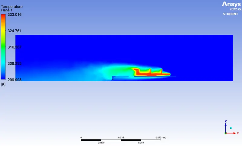
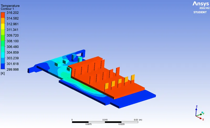
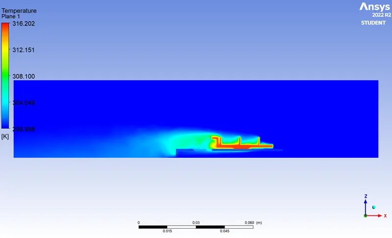
Temperature Contour
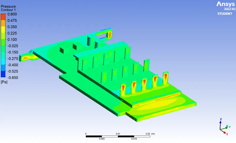
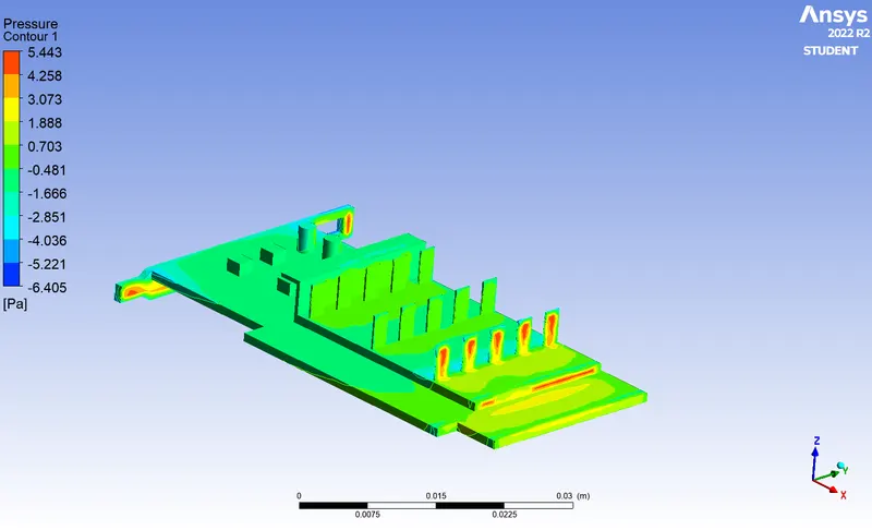
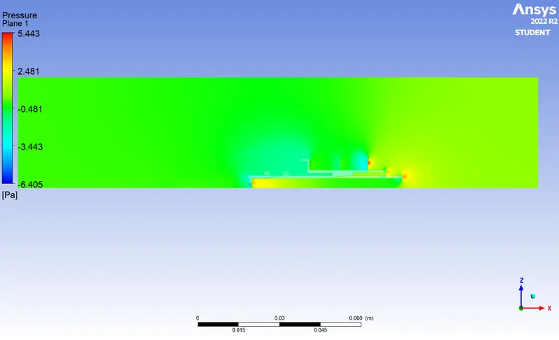
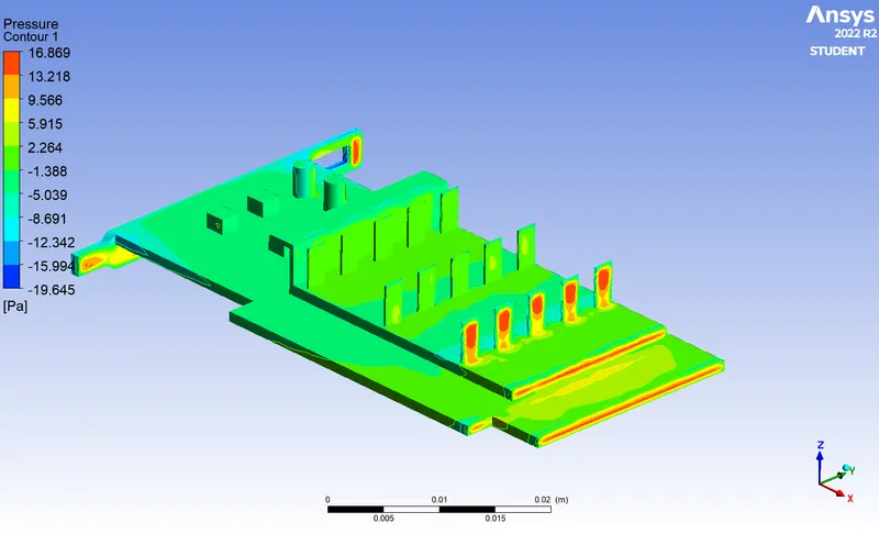
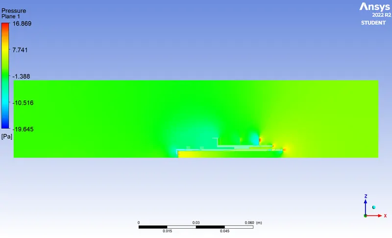
Pressure Contour
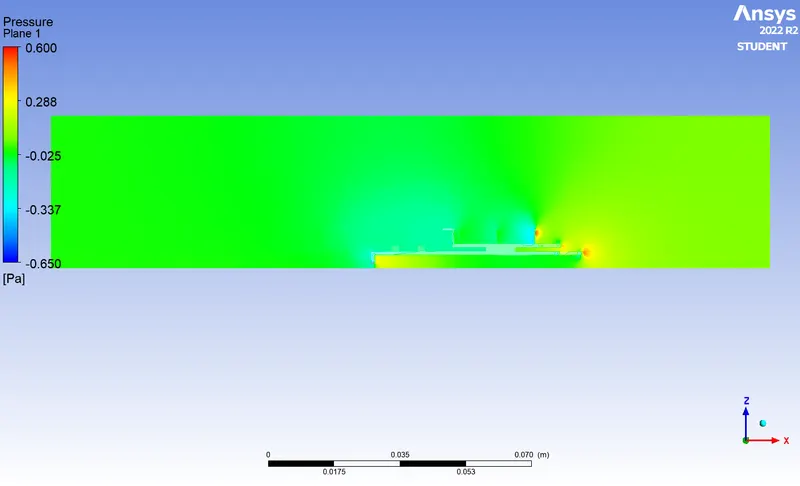
Case : 2 For fluid flow velocity of 3 m/s
Residulas
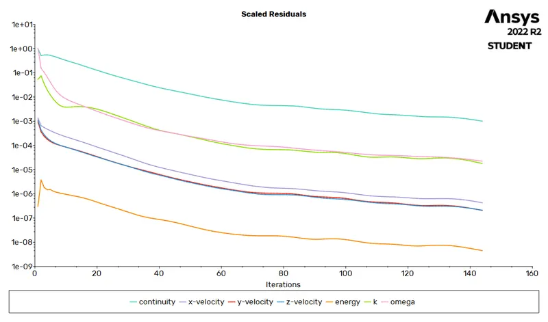
Heat Transfer Coefficient
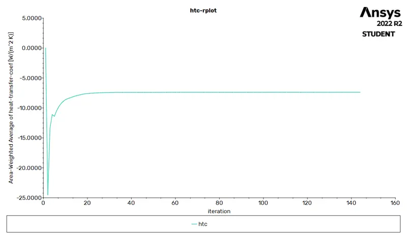
Maximum Temerature of The Processor
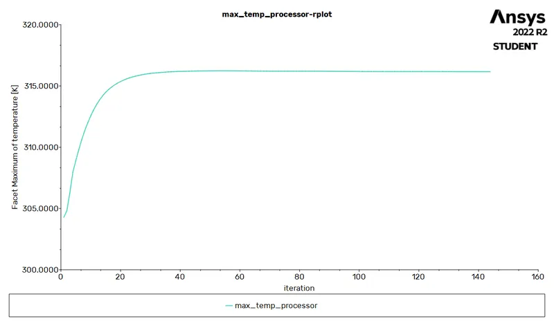
Temperature Contour
Pressure Contour
Case : 3 For fluid flow velocity of 5 m/s
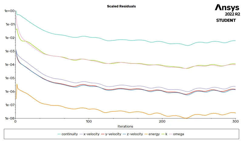
Residulas
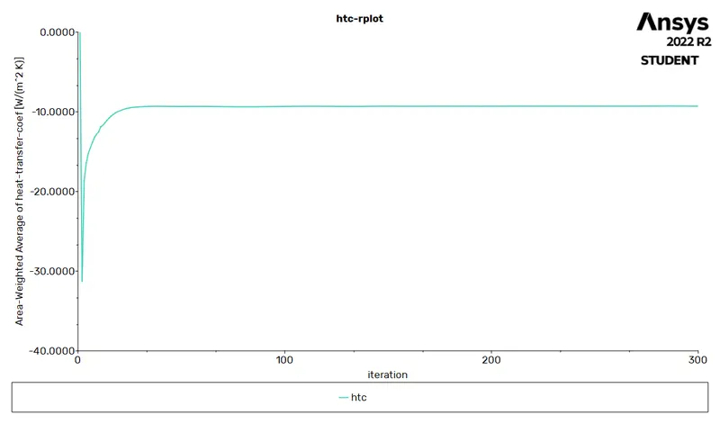
Heat Transfer Coefficient
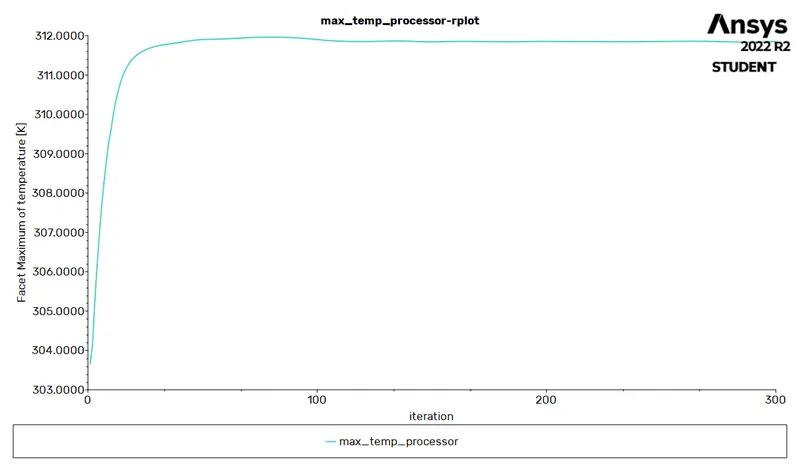
Maximum Temerature of The Processor
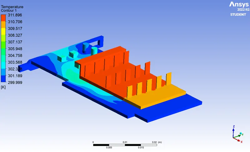
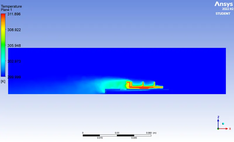
Temperature Contour
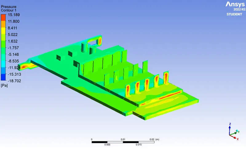
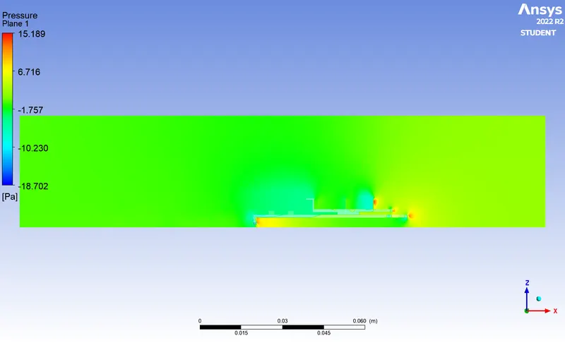
Pressure Contour
Case : 4 For fluid flow velocity of 3 m/s (Refined mesh)
Residulas
Heat Transfer Coefficient
Maximum Temerature of The Processor
Temperature Contour
Pressure Contour
Case : 5 For fluid flow velocity of 5 m/s (Refined mesh)
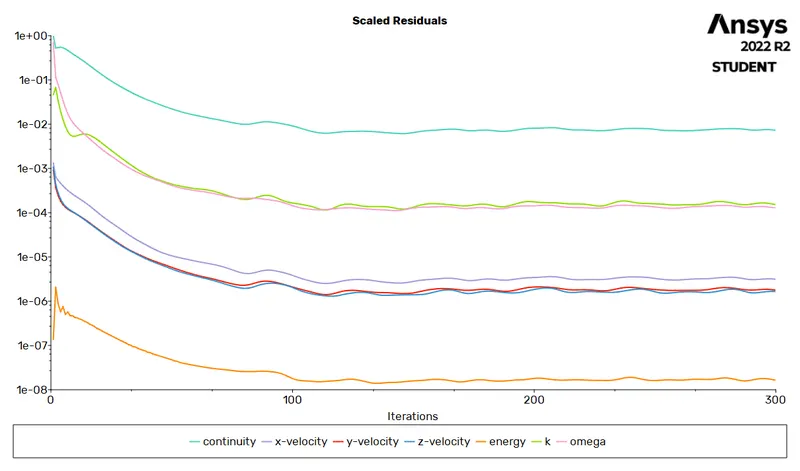
Residulas
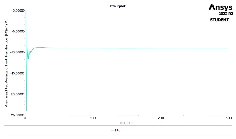
Heat Transfer Coefficient
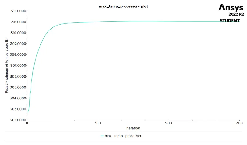
Maximum Temerature of The Processor
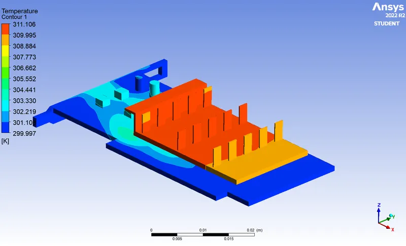
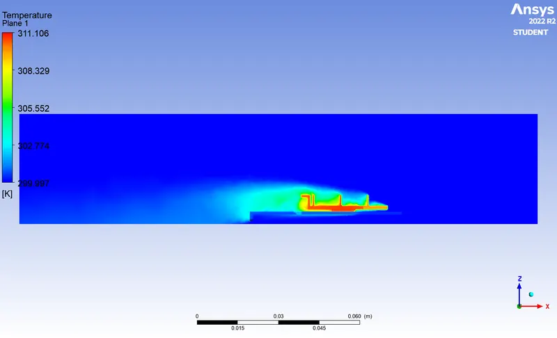
Temperature Contour
Pressure Contour
Conclusion
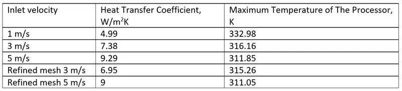
Temperature of the processor is maximum for the inlet velocity of 1 m/s and heat transfer coefficient is maximum for the inlet velocity of 5 m/s. The negative sign indicates that the heat is leaving.
It has been observed that the temperature decreases while velocity of the fluid flow increases.
Heat transfer coefficient increases when velocity of the fluid flow increases.
For refined mesh case results are very much close compared with coarse mesh and are able to validate the results accurately.