Week 5 - Genetic Algorithm

Stalagmite Function

function [f] = stalagmite(input_vector)

x = input_vector(1);
y = input_vector(2);

t1 = (sin((5.1*pi*x)+0.5))^6;
t2 = (sin((5.1*pi*y)+0.5))^6;
t3 = exp(-4*log(2)*((x-0.0667)^2)/0.64);
t4 = exp(-4*log(2)*((y-0.0667)^2)/0.64);

f = -(t1*t2*t3*t4);
end

Coding genetic algorithm for this stalagmite function

clear all
close all
clc

%Definie our search space
x = linspace(0,0.6,150);         %x array
y = linspace(0,0.6,150);         %y array
n = 50;                          %number of cases

%Creating a 2D mesh
[xx yy] = meshgrid(x,y);

%Evaluating a stalagmite function
for i = 1:length(xx)
    for j = 1:length(yy)
        input_vector(1)=xx(i,j);
        input_vector(2)=yy(i,j);
        f(i,j) = Stalagmite(input_vector);
    end
end

%Study 1 : Statistical Behaviour

tic
for i = 1:n
    [inputs,fopt(i)] = ga(@Stalagmite,2);
    xopt(i) = inputs(1);
    yopt(i) = inputs(2);
end
study1_time = toc

figure(1)
subplot(2,1,1)
hold on
surfc(xx,yy,-f)
shading interp
xlabel('X-axis')
ylabel('Y-axis')
title('Statistical Behaviour with Unbound inputs')
plot3(xopt,yopt,-fopt,'marker','o','markersize',5,'markerfacecolor','r')
subplot(2,1,2)
plot(-fopt)
xlabel('No. of Iterations')
ylabel('Function maximum')

%Study2 : Statistical behaviour with upper and lower bounds

tic
for i = 1:n
    [inputs,fopt(i)] = ga(@Stalagmite,2,[],[],[],[],[0;0],[1;1]);
    xopt(i) = inputs(1);
    yopt(i) = inputs(2);
end
study2_time = toc

figure(2)
subplot(2,1,1)
hold on
surfc(xx,yy,-f)
shading interp
xlabel('X-axis')
ylabel('Y-axis')
title('Statistical behaviour with upper and lower bounds')
plot3(xopt,yopt,-fopt,'marker','o','markersize',5,'markerfacecolor','r')
subplot(2,1,2)
plot(-fopt)
xlabel('No. of Iterations')
ylabel('Function maximum')

%Study3 : Statistical Behaviour with increasing iterations of GA

options = optimoptions('ga');
options = optimoptions(options,'PopulationSize',300);

tic
for i = 1:n
    [inputs,fopt(i)] = ga(@Stalagmite,2,[],[],[],[],[0;0],[1;1],[],[],options);
    xopt(i) = inputs(1);
    yopt(i) = inputs(2);
end
study3_time = toc

figure(3)
subplot(2,1,1)
hold on
surfc(xx,yy,-f)
shading interp
xlabel('X-axis')
ylabel('Y-axis')
title('Statistical Behaviour with increasing iterations')
plot3(xopt,yopt,-fopt,'marker','o','markersize',5,'markerfacecolor','r')
subplot(2,1,2)
plot(-fopt)
xlabel('No. of Iterations')
ylabel('Function maximum')

Output

figure(1)

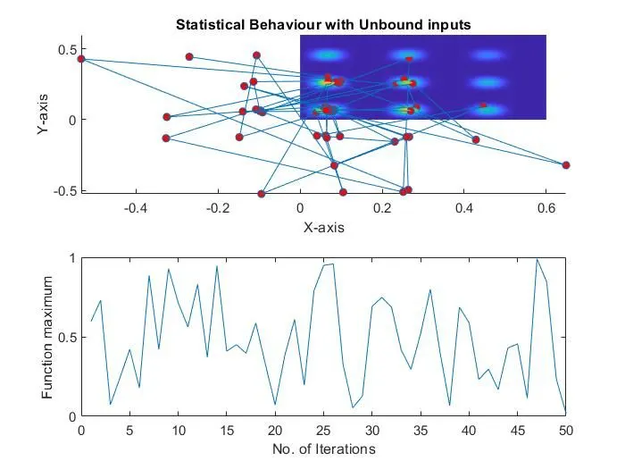
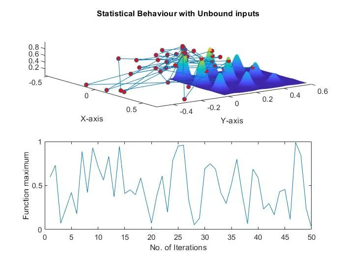
1. The plot3 command is used to make a plot of xopt,yopt and -fopt in order to plot the optimum maximas.

2. Study time = 3.675

figure(2)

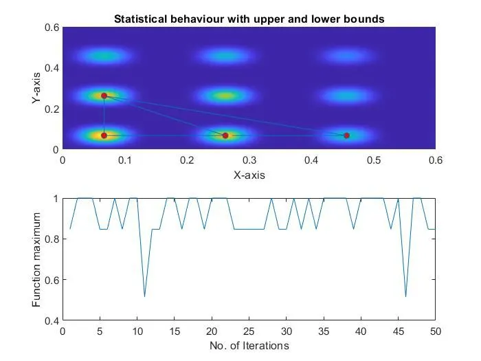
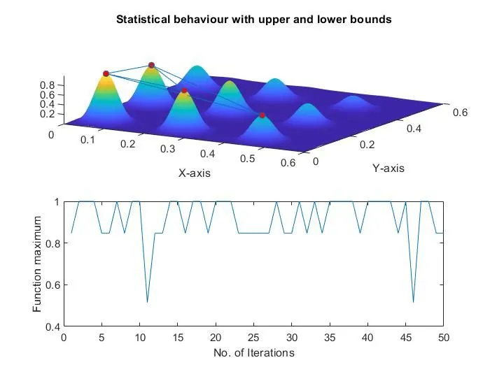
1. Lower and upper bounds are specified for x and y and the ga is initiated with radom population.

2. Study time = 4.38

figure(3)

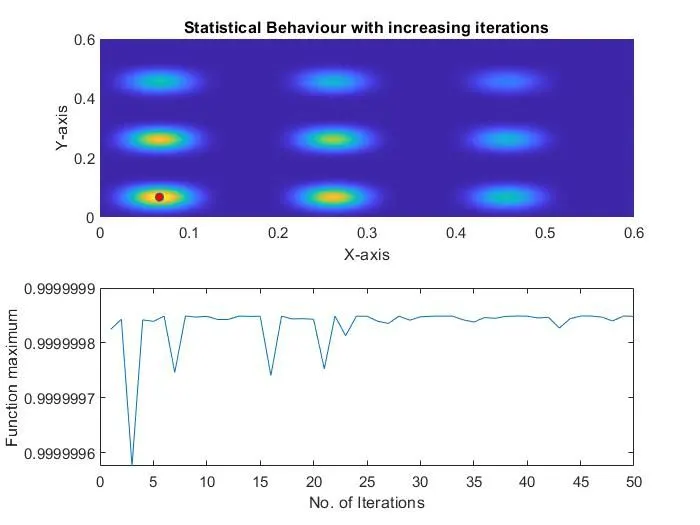
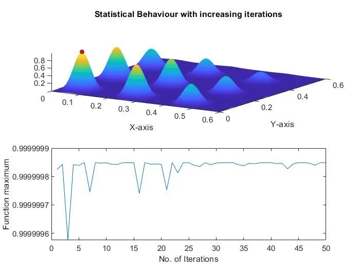
1. In this 3 rd study, the number of iterations is increased to 300 to converge and find the global maxima of the function.

Here we can see that there is only one red dot on the stalagmite function and that is the required global maxima point.

2. To get the time taken to complete the cycle tic toc command is used to record the time.

3. Study time = 15.047

4. By increasing the population size of the ga we can increase the accuracy of the algorithm.

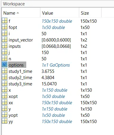
Workspace output:

Reference

1. https://in.mathworks.com

2. https://skilllync.com