Week 6 - CHT Analysis on a Graphics card

Objective: To perform a steady state conjugate heat transfer analysis on a model of graphics card.

introduction

The term conjugate heat transfer (CHT) describes the process which involves variation of temperature within solids and fluids, due to thermal interaction between the solids and fluids, the exchange of thermal energy between the two physical bodies is called study of heat transfer, the rate of transferred heat is directly proportional to the temperature difference between the bodies.

Conjugate heat transfer corresponds with the combination of heat transfer in solid and heat transfer in fluids, in solids, conduction often dominates whereas in fluids, convection usually dominates. efficiently combining heat transfer in fluids and solids is key to designing effective coolers, heaters or heat exchanger. forced convection is the most common way to achieve high heat transfer rate. in some applications the performances are further improved by combining convection with phase change.

Heat transfer in solids and heat transfer in fluids are combined in the majority of applications. this is because fluids flow around solids or between solid walls and because solids are usually immersed in a fluid.

Graphic card

A graphics card (also called a display card, video card, display adaptor or graphics adaptor) is an expansion card which generates a feed of output images to a display device like monitor. the graphics card is responsible for rendering an image to your monitor. it does this by converting data into a signal which your monitor can understand.

Geometry 

• Download and import model in geometry.
  
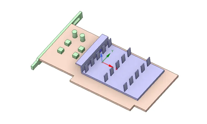
• Share topology to make sure that we get conformal mesh.

Meshing

The cut section plane is shown below

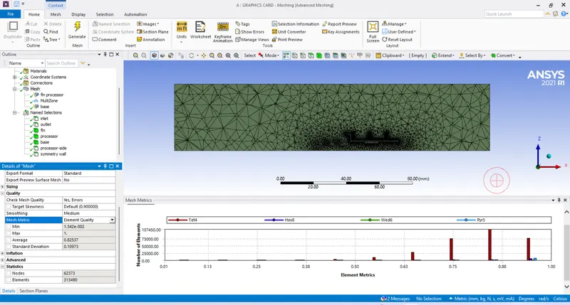
The overall mesh quality is good.

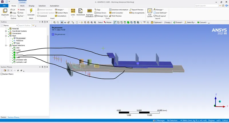
The named section for body is shown below

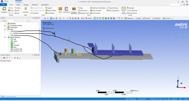
The body sizing and multizone are shown below

The multizone for hex mesh are applied to fin and processor body

The mesh details are shown below

a) For enclosure the mesh size = 8 mm

b) For fin and processor the element size = 0.5 mm

c) For base the element size = 1 mm

Setup

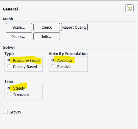
• general setup
  • solver type: pressure based
  • velocity formulation: absolute
  • time: steady state
    
  • Enable energy.
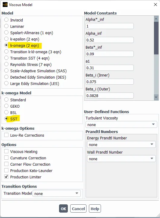
  • Turbulence model: K-Omega SST
    
• Materials
  • copy solid materials from fluent data base.

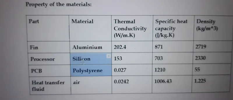
The base,fin and processor are need to be set by Polystyrene, Aluminium and Silicon respectively.

The material properties to be set as shown below.

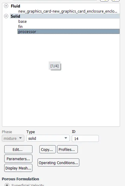
Enable cell zone under fluid and solid respectively

Enable source term for processor and set value 15625000`W/m^3`.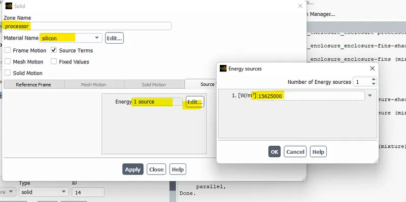

Case 1

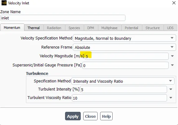
a) Set velocity inlet = 5 m/s.

• •  Boundaries
    • inlet 
      • type: velocity inlet, 
         
        • Outlet 
          • Type: pressure outlet
          •  Symmetry
            • type: symmetry

• Initialize
  • hybrid initialization.
• Create contour for temperature.
• Run simulation.

RESULTS

1) At velocity 5 m/sec

a)Mesh details for coarse mesh

a) For enclosure the mesh size = 8 mm

b) For fin and processor the element size = 0.5 mm

c) For base the element size = 1 mm

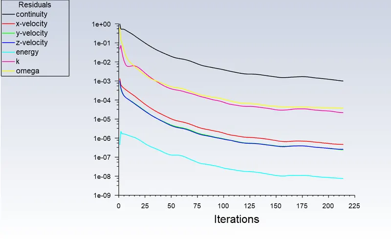
Scaled Residual

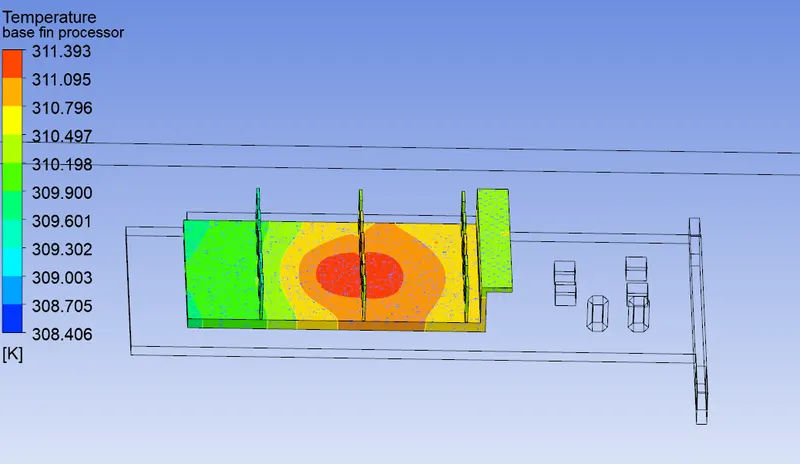
The temperature distribution for fins and processor are shown below

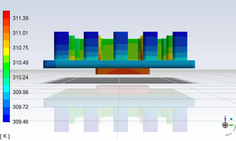
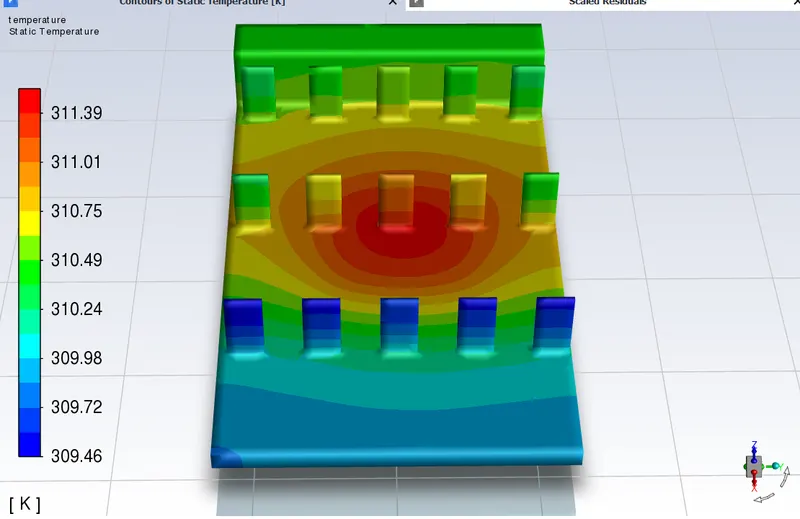
From this contour, it is clear that the maximum temperature is at processor as it is a heat generating source. The black coloured shaded area(Blue colour contour) is having low temperature because it is exposed to air and there is 2 dimensional conduction along the length of the fin base as shown below.

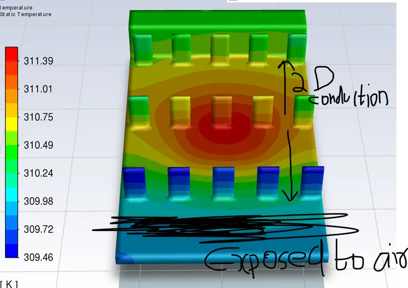
The green colour contour is in other direction because the fin on front blocks the air and it not reaching at back side. So, any reduction in temperature at back side is due to 2 dimensional heat conduction only.

Let's look at the processor only.

The area attached to base have maximum temperature because it is attached to non conducting base.

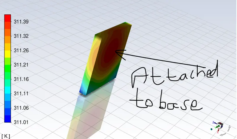
The maximum temperature at any point on this surface is 311.39 K and area weighted average at this surface is 311.29 K.

The temperature distribution along the thickness is parabolic as per theory and we are having minimum area weighted average temperature of 311.24 K at the fin-processor interface. This is mathematically correct as per equation in Incropera textbook.

So, the area of processor attached base is the potential hotspot in this model. It is true as per theory also.

The Volume average heat transfer coefficient for processor is -269.24993 W/m2K.

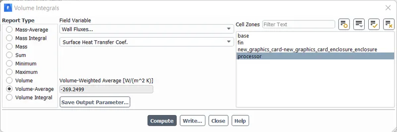
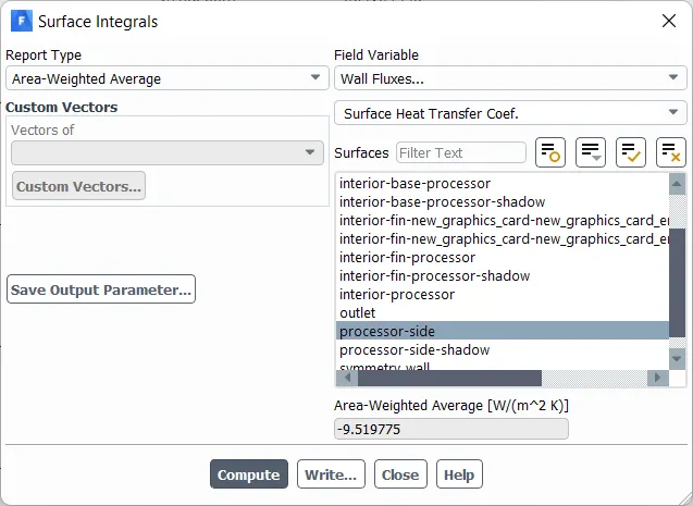
But it is more convenient to take the average heat transfer coefficient at the side wall of the processor as it is exposed to the outside air. The value is -9.519775 W/m2K.

The temperature distribution from CFD post for fin and processor are shown below

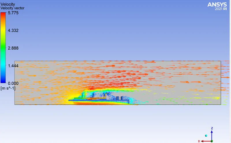
The velocity vector plot is shown below

b) Fine mesh

b) Reducing mesh size such that I m reducing mesh size of the processor and fin as this is the area of interest

The hex mesh size is reduced to 0.25 mm

The cell count is increased

Run Simulation

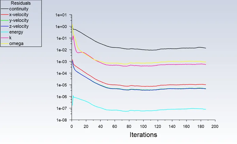
Scaled Residual

The maximum temperature is at base-processor interface 311.14638 K.

The area weighted average of heat transfer coefficient at side wall of processor is -8.986778 W/m2K.

2) At velocity 3 m/sec

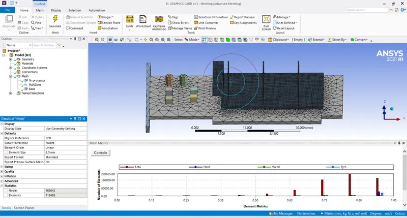
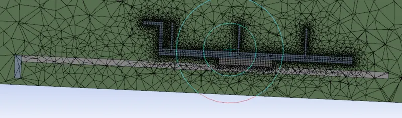
I use fine mesh size of 0.25 mm for fins and processor here as it gives more accurate result.

I m increasing the mesh size for base to 5 mm as it is irrelevent here and to reduce the cell count.

The mesh is shown below

Open set up and change the velocity at inlet to 3 m/s

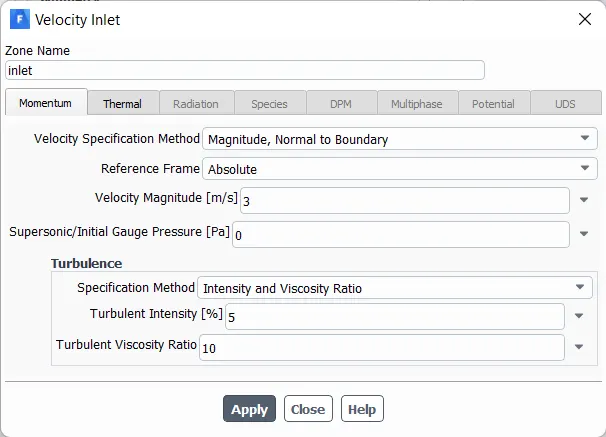
Run Simulation

Scaled Residual

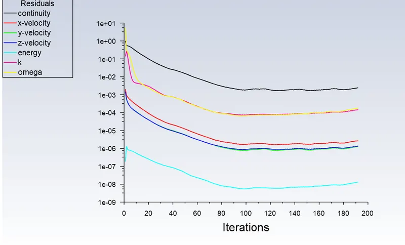
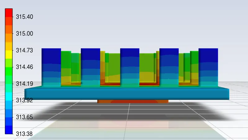
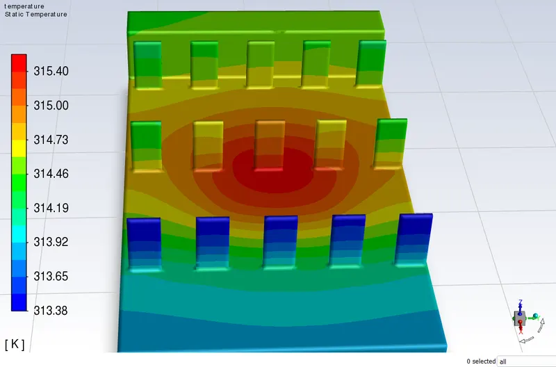
The maximum temperature is at base-processor interface 315.3003 K.

The area weighted average of heat transfer coefficient at side wall of processor is -8.009309 W/m2K.

The temperature distribution for fins and processor are shown below

---------------------------------------------------------------------------------------------------------------------------------------------------------

3) At velocity 1 m/sec

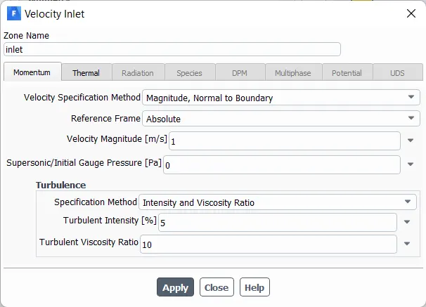
Open set up and change the velocity at inlet to 1 m/s

Run Simulation

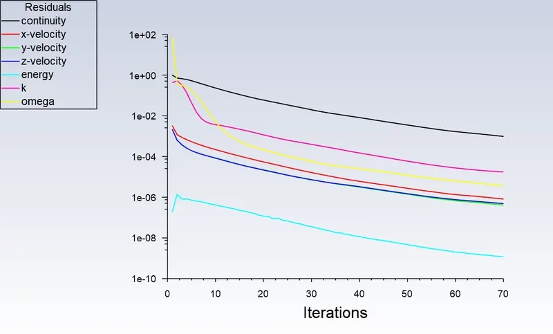
Scaled Residual

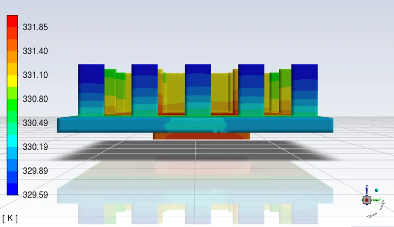
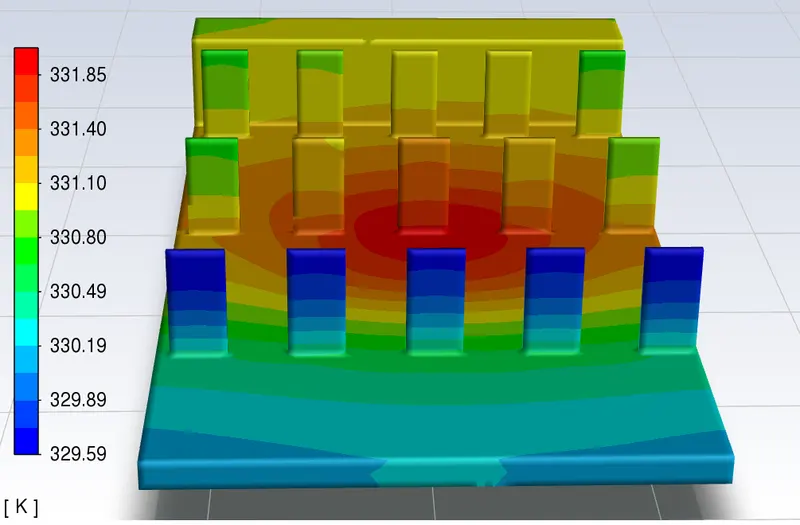
The maximum temperature is at base-processor interface 331.7498 K.

The area weighted average of heat transfer coefficient at side wall of processor is -5.213341 W/m2K.

The temperature distribution for fins and processor are shown below