Week 6 - CHT Analysis on a Graphics card

Aim- To create a Conjugate Heat transfer coefficient on a Graphics card and find an effect of temperature with varying velocity on a graphics card processor.

Objective-

• To perform a steady state conjugate heat transfer analysis on the graphics card.
• To find the maximum temperature and heat coefficient attended by the processor.
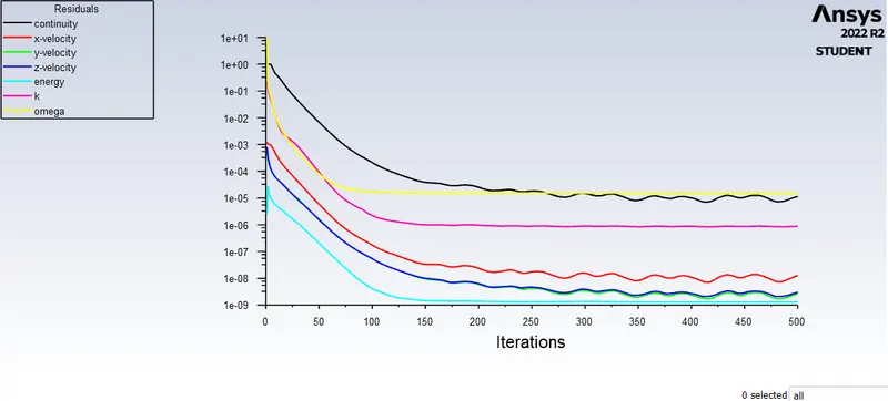
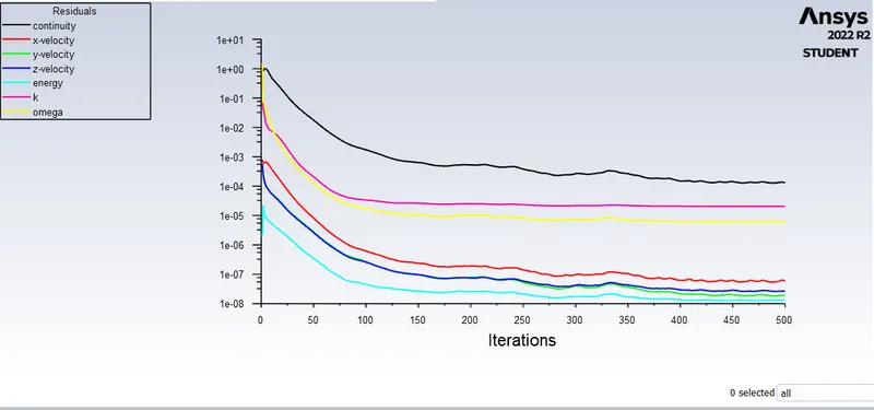
• Prove the convergence point on the simulation with appropriate plots and images.
• And point out the official hotspot obtained on the graphics card.

Theory-

Conjugate heat transfer-

The Conjugate Heat Transfer (CHT) analysis type allows for the simulation of heat transfer between solid and fluid domains by exchanging thermal energy at the interfaces between them. Typical applications of this analysis type exist as, but are not limited to, the simulation of heat exchangers, cooling of electronic equipment, and general-purpose cooling and heating systems.

It provides a temperature predictions and thermal hotspots of solid -fluid interface and it helps to predict the heat transfer accurately. It also provides velocity and pressure distribution of fluid moving inside the solid. By this the CHT help to open a door for imporvemnt of design for better heat transfer and cooling capacity.

A Graphic card or video card is used to in computers and works as a external card that generates and give visual information on the screen of the system. It contains a processor which unloads some load from the main processor. For the thermal efficiency and heat transfer on the processor it consists of some fins and current generation graphics card also comes with integrated fans. To run a simulation in any CFD/CAD software graphics is very preferable.

Geometry-

• Import the geometry of a graphics card onto the Spacecalim geometry on the Ansys workbench.

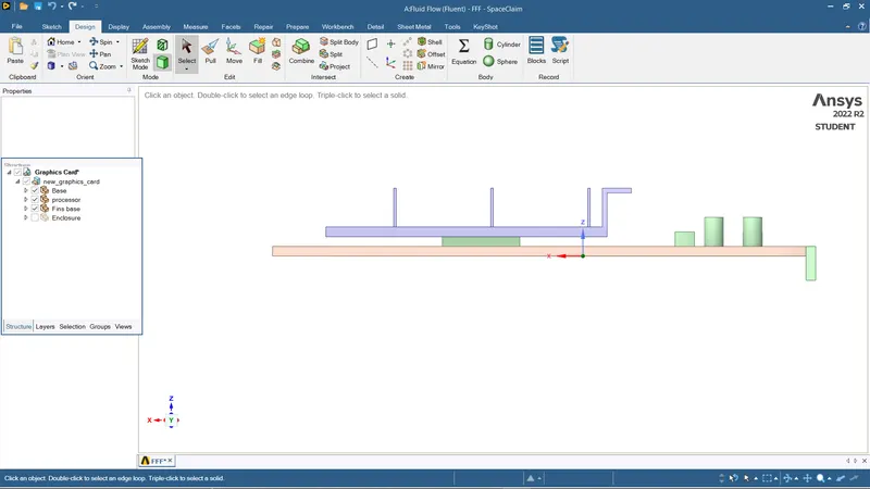
• Identify every component of the geometry.

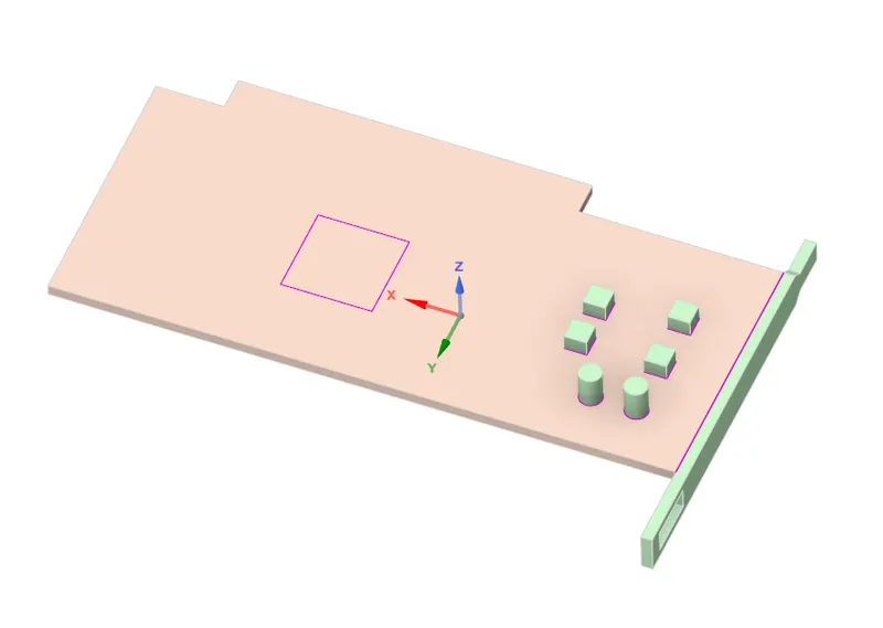
Base of the graphics card

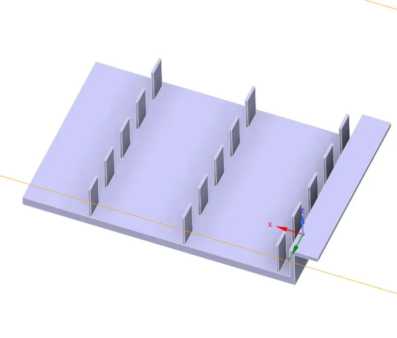
Fins of the graphics card

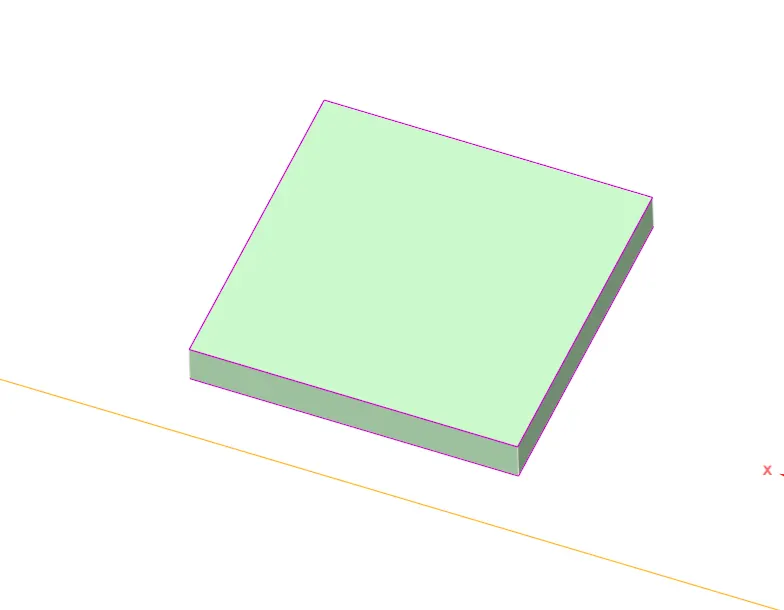
processor of the graphics card

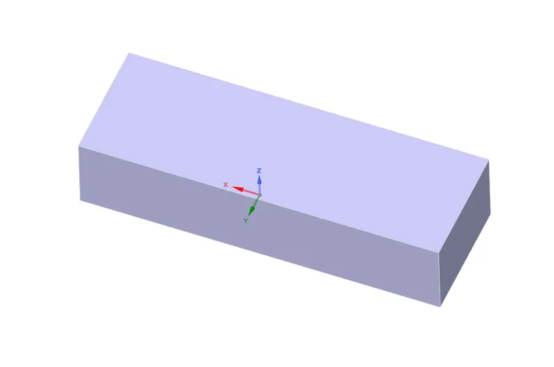
Enclosure around the graphics card for the simulation

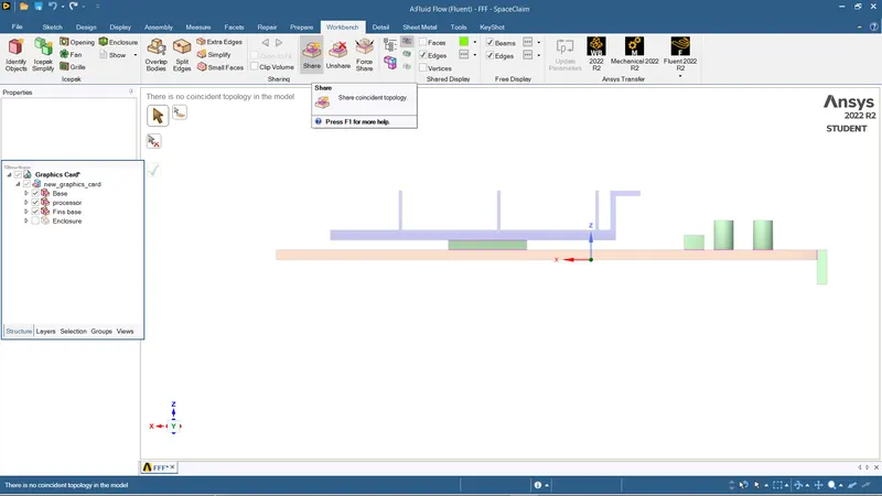
• check share topology of the geometry and enable the share Topology feature form the above operations on the SpaceClaim interface this helps to create a good mesh of the geometry without having any intersection between the mesh.

Meshing-

• Named each part of the geometry for the convenience while setting up the simulation.

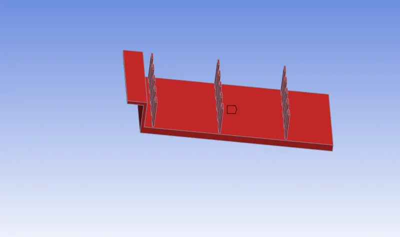
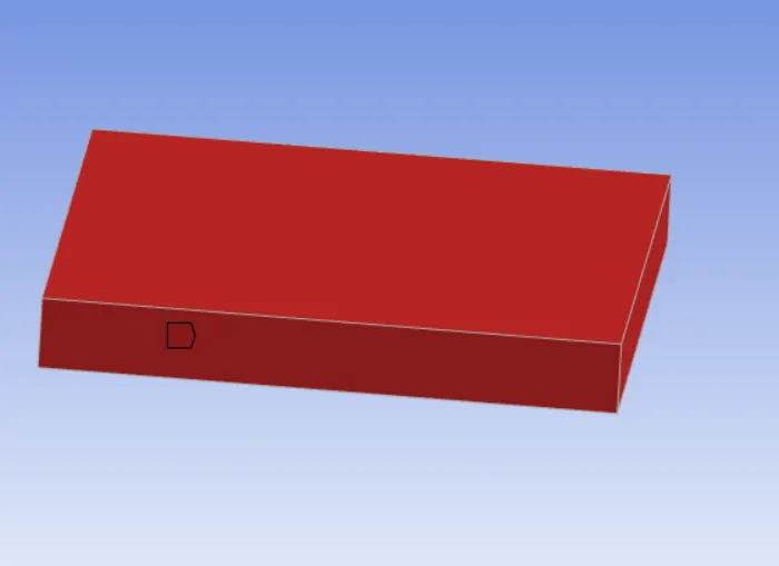
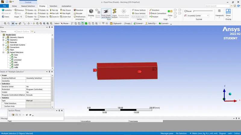
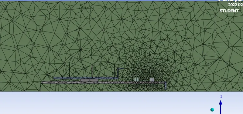
We ran a baseline mesh to identify and understand the constraints and we also ran this simulation with the baseline mesh itself. It will work as guideline to develop a refined mesh for further getting a accurate simulation results

Setup-

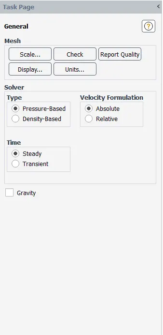
we use a pressure-based type solver with velocity formulation as absolute and we ran a Steady-state simulation.

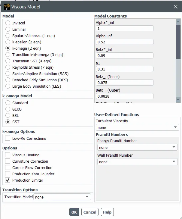
For the viscous model we go with K-Omega(2 eqn)

For the assigning of materials to the geometry, some materials have been created,

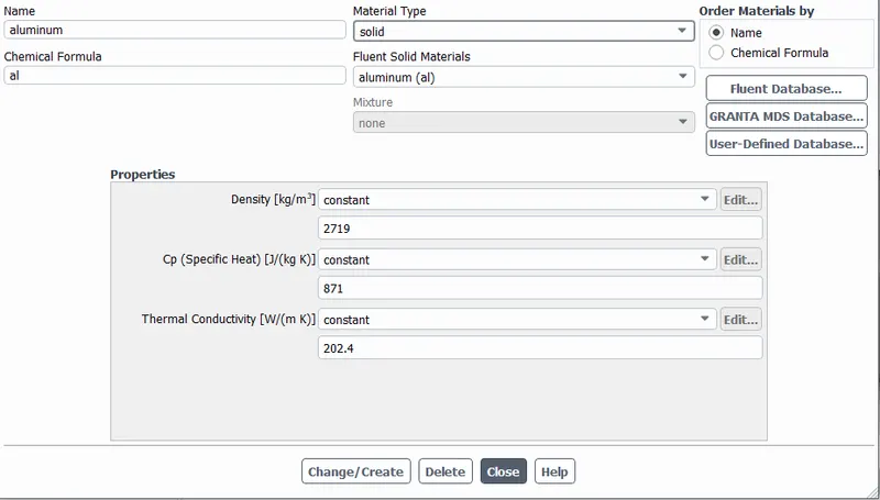
Aluminum-----Fins

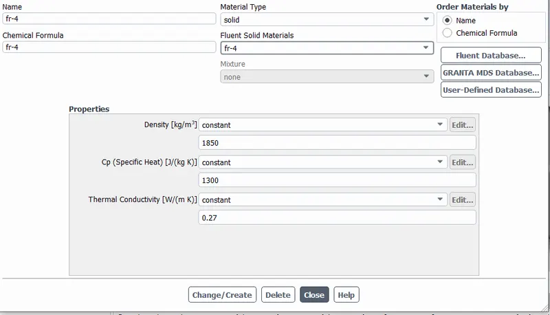
Fr-4----------Base

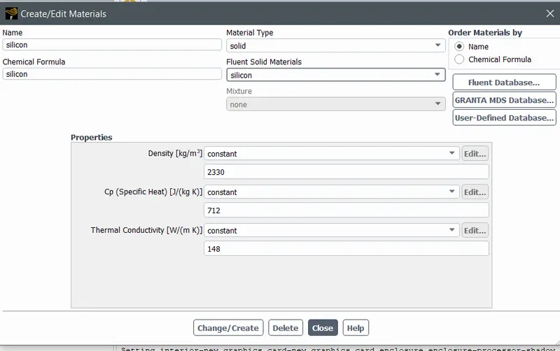
Silicon-------Processor

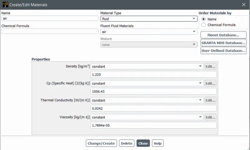
Air----------Enclosure

Thermal properties of the following materials-

Fins

Base

Processor

Air

We have assign the respective materials to the respective body for the analysis using Cell zone conditions.

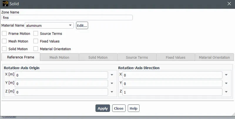
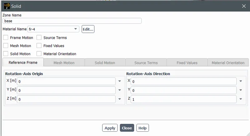
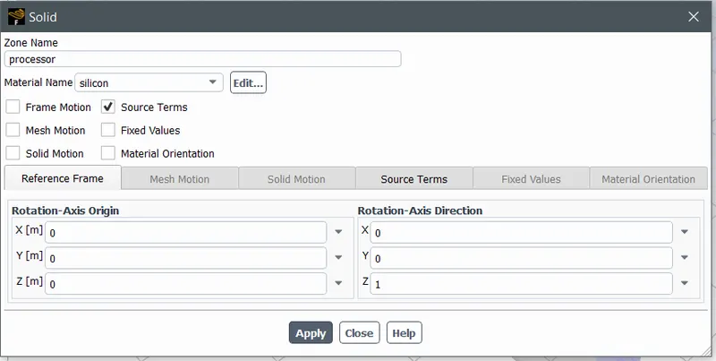
As we know that the heat source is a processor so, we have provided a heat source on the processor

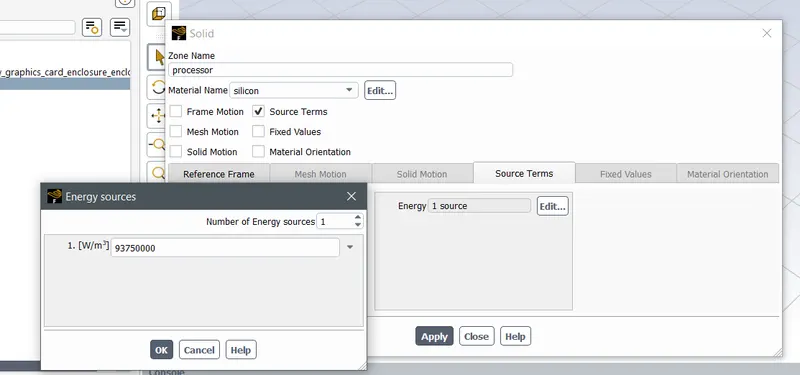
We have used 6W processor so,

volume of the processor-6.4*10^-8

so, Heat generated= Power/Volume

=6/6.4*10^-8 =93750000

Report-

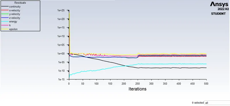
Temperature

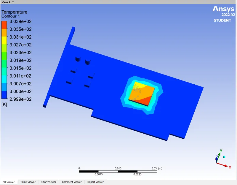
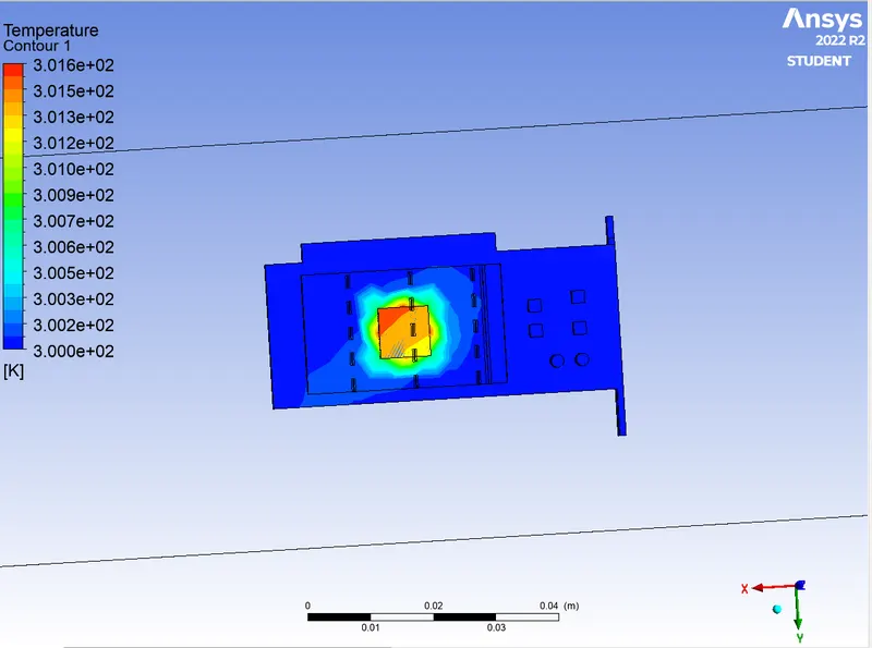
Global Hotspots

Wall Adjacent Temperature

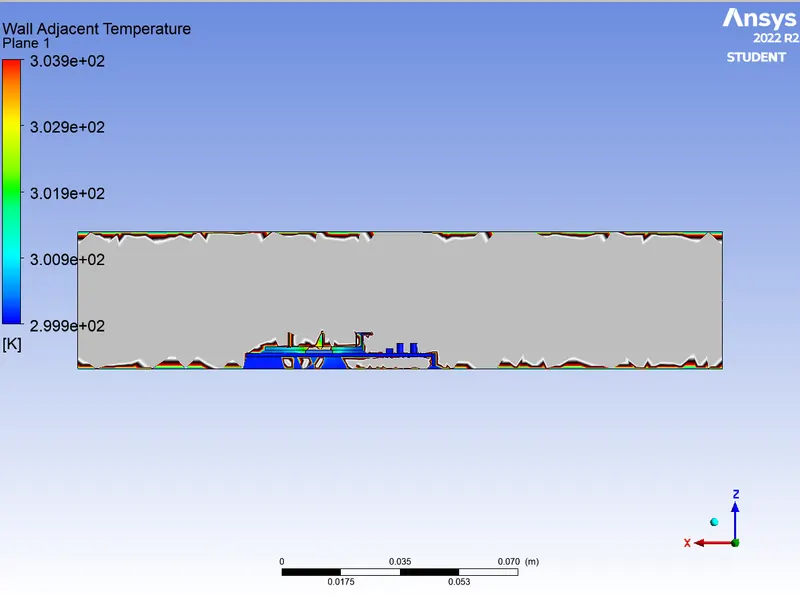
As we can see that some entities readings are not been captured fluently. So lets perform the same calculation with a refined mesh and with some changing boundary conditions i.e 1m/s, 3m/s, 5m/s.

Refined mesh-

we go with the element sizes as--

Enclosure- 1.8mm

processor - 1mm

Base- 1mm

Fins- 1mm

The enclosure mesh element size is greater than the other three entities because we want to capture the change in temp, and velocity on the processor, base, and fins with respect to the inlet boundary conditions.

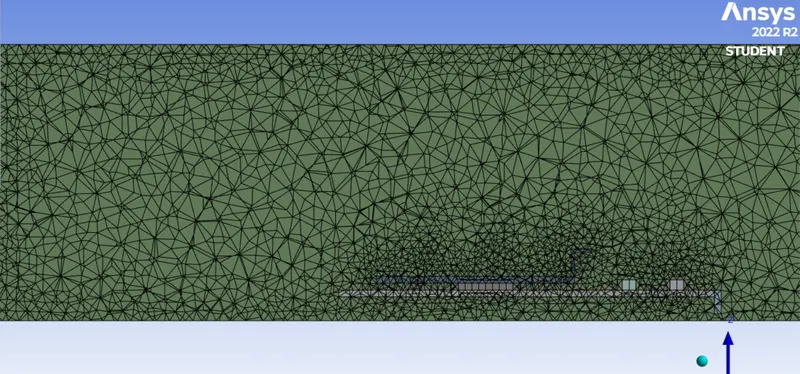
we used the sizing method to define the meshing constraints on the Base, Processor, and Fins.

Refined mesh elements statistics.

Setup-

So after performing a refined mesh on the geometry we perform the same fluent analysis as previous but we will try to calculate and compare the variations in result with varying inlet boundary conditions.

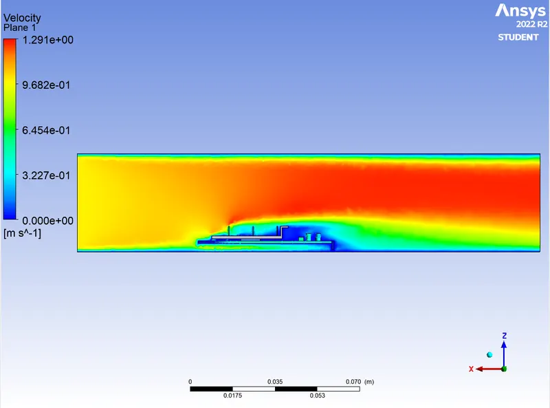
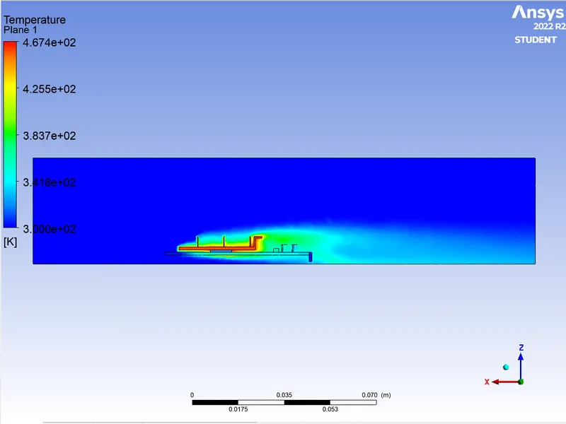
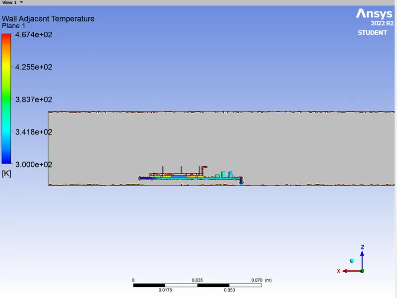
Case-1 - inlet boundary conditions=1m/s

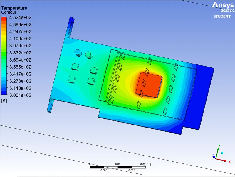
Global Hotspot Region

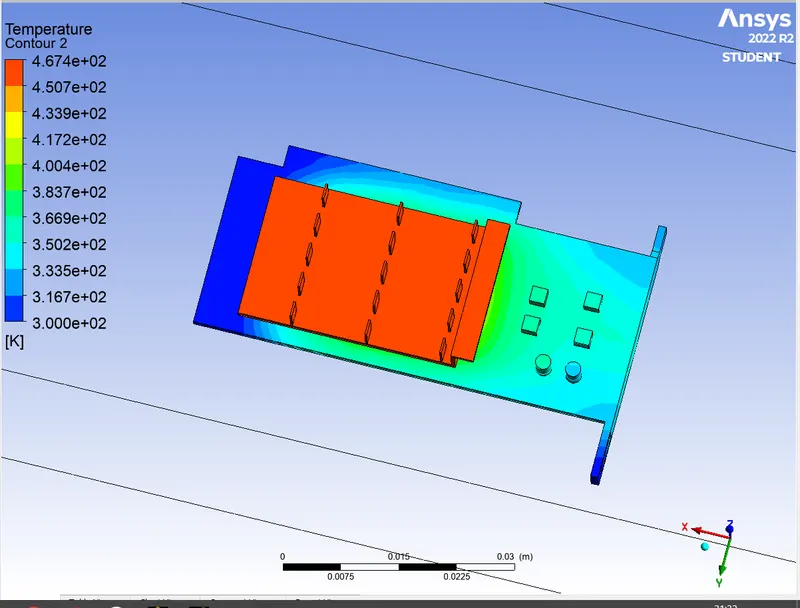
Temperature on the processor

Velocity Plane

Temperature Plane

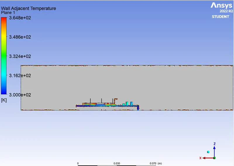
Wall Adjacent Temprature

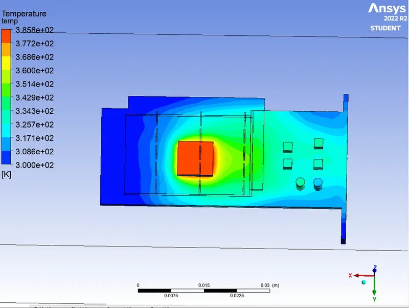
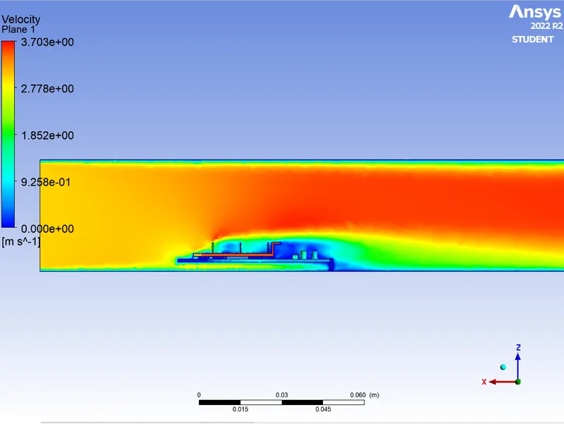
Case-2 Inlet Boundary Conditions=3m/s

Global Hotspot Region

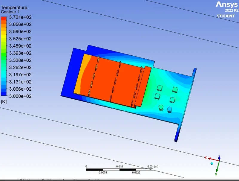
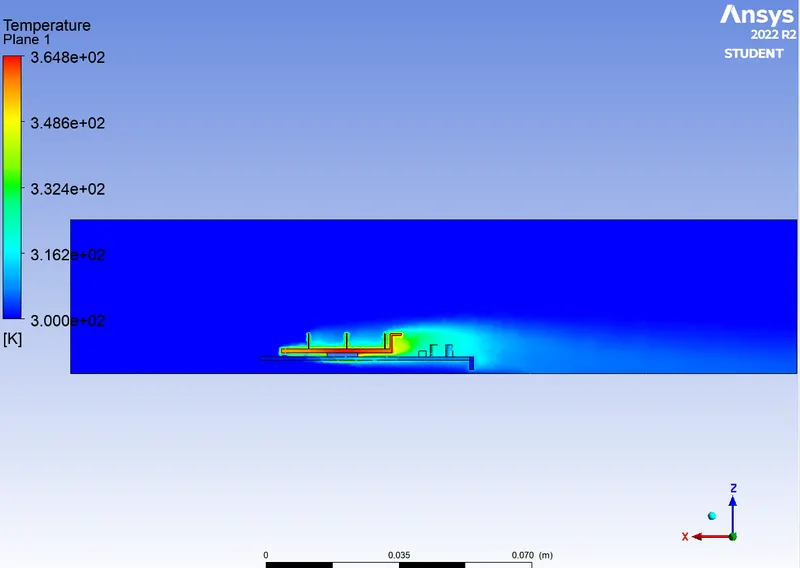
Temperature on the processor

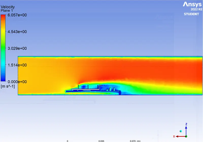
Velocity plane

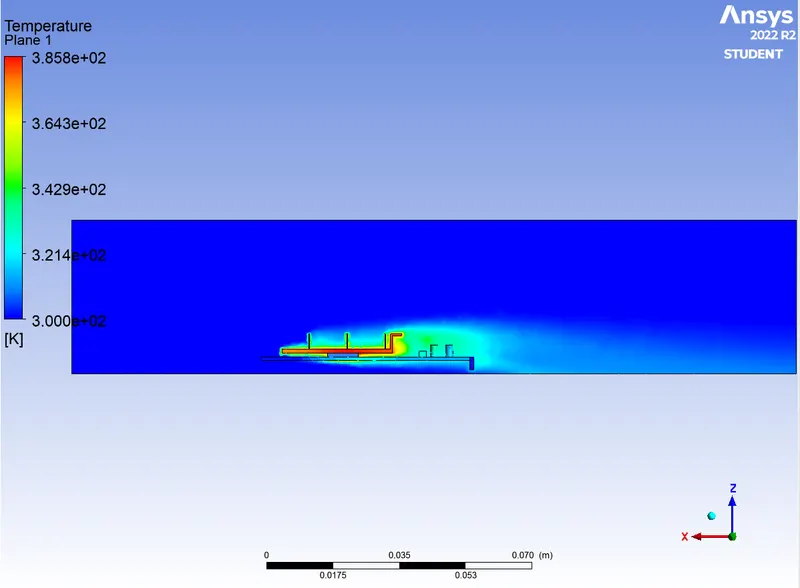
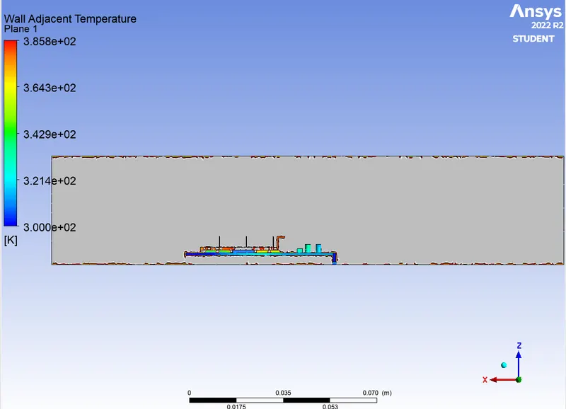
Case-3 Inlet Boundary Conditions= 5m/s

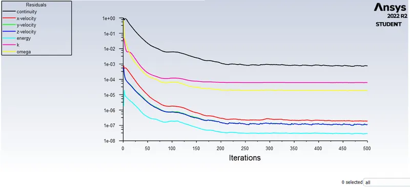
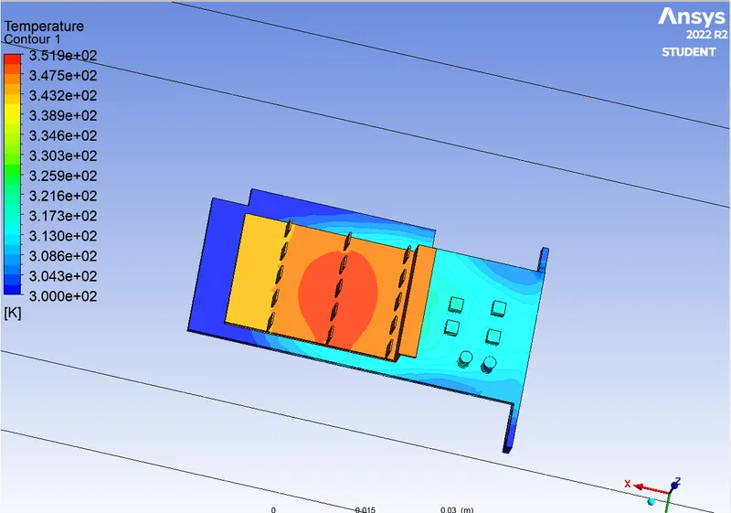
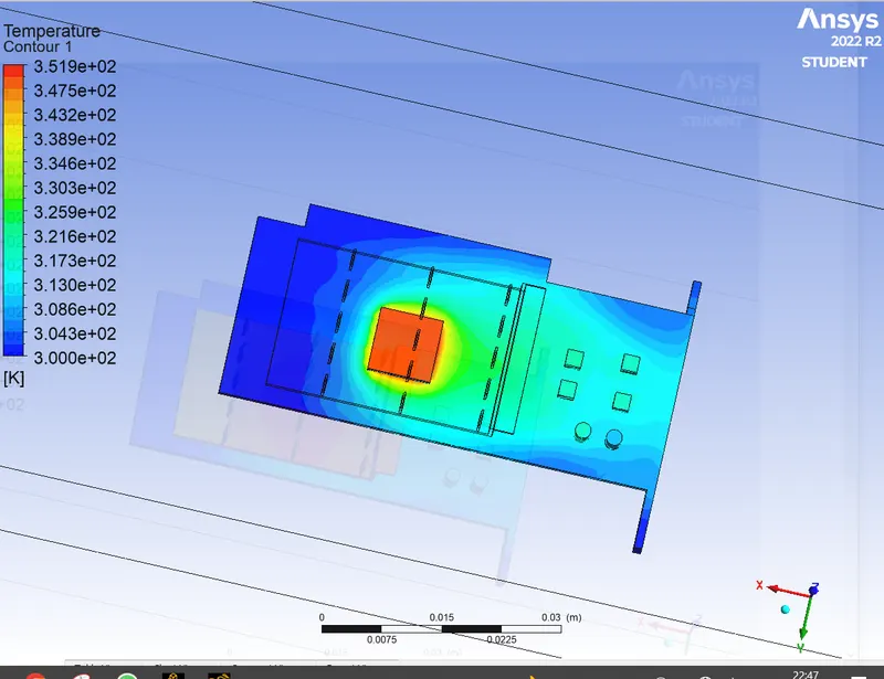
Results-

Velocity	Temperature at Processor (k)	Temperature at Fins(k)	Heat Transfer Coefficient(w/m^2K)
1 m/s	466.73 k	462.19 k	133 w/m^2k
3 m/s	385.14 k	380.68 k	139 w/m^2k
5 m/s	364.25 k	359.81 k	147 w/m^2k

Conclusions-

• From the above analysis, we can understand that as the number of elements increases the accurate analysis of temperature distribution is obtained.
• As the inlet velocity increases the net temperature on the graphic card component decreases.
• Hence it can be concluded with a statement that the higher inlet velocity results in better cooling of the components while lowering the temperature of the components and hence it will also increase the efficiency of the work and keep the components safe from damage.