Week 6 - CHT Analysis on a Graphics card

CHT Analysis on a Graphics card

AIM:

• Perform a steady-state conjugate heat transfer analysis on a graphics card model.
• Run the simulation for the best possible mesh with a combination of coarse and refined mesh in different regions. Explain the reason for choosing the particular mesh settings.

OBJECTIVES:

• Run the simulation by varying the velocity from 1m/sec to 5m/sec for at least 3 velocities and discuss the results.
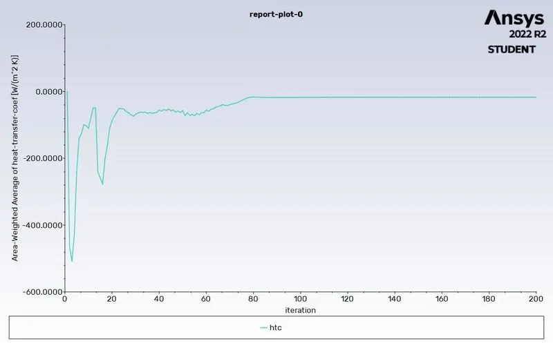
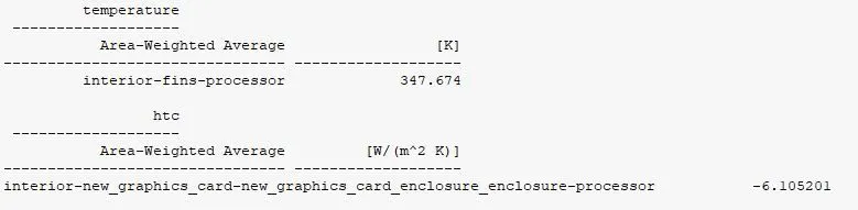
• Find out the maximum temperature and the average heat transfer coefficient attained by the processor.
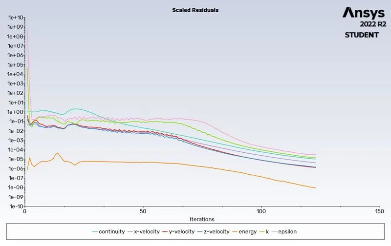
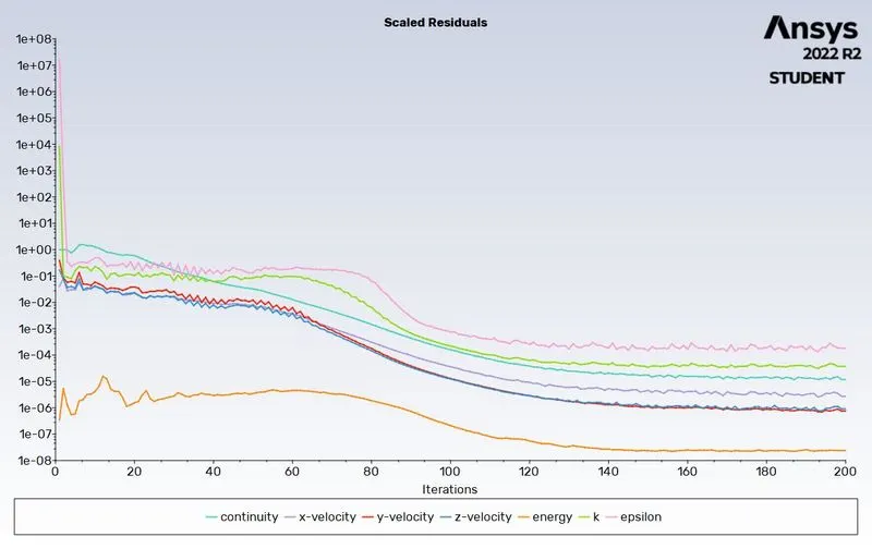
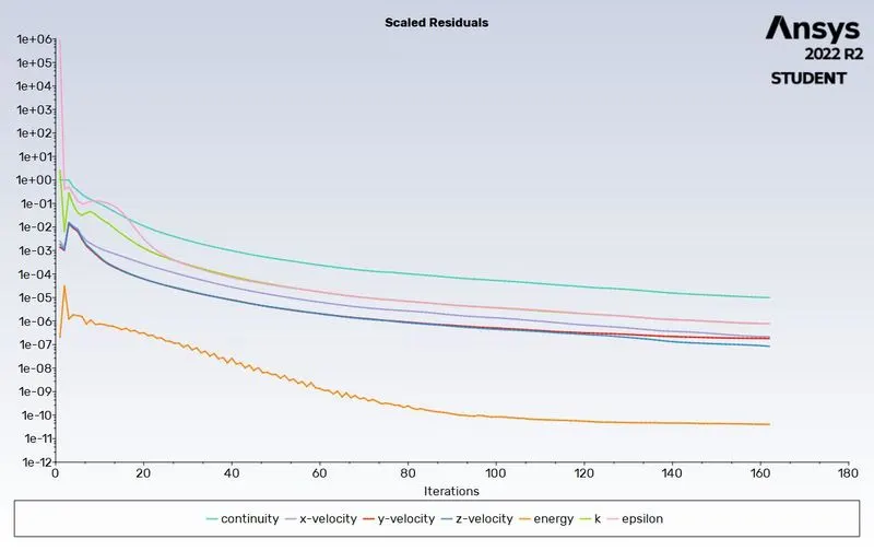
• Prove that the simulation has achieved convergence.
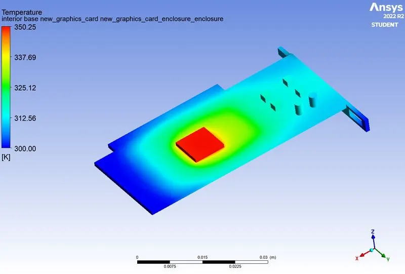
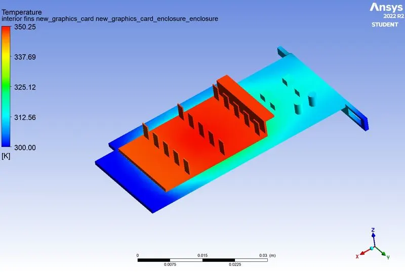
• Identify potential hotspots on the model.

THEORY:

Conjugate Heat Transfer(CHT) is the combination of both conduction and convection. It is mainly observed when heat transfer occurs between a solid body and fluid flow. Typical examples in which we can observe CHT are heat exchangers, cooling of electronic equipment, and general-purpose cooling and heating systems.

In this analysis, we are conducting a steady-state conjugate heat transfer (CHT) analysis on a Graphics card model. Graphics cards are one of the most used electronic components in personal computers and workstations. As they are used primarily for tasks that need heavy usage, they get heated up pretty quickly and that might lead to power losses. In order to prevent such losses, we need to identify the hot spots and provide some measures for better cooling. Running the graphics card at an optimal temperature reduces the power loss and increases the product's performance and life.

MODELLING APPROACH:

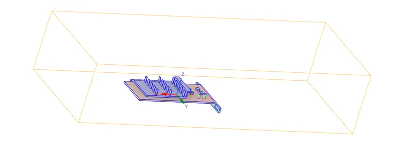
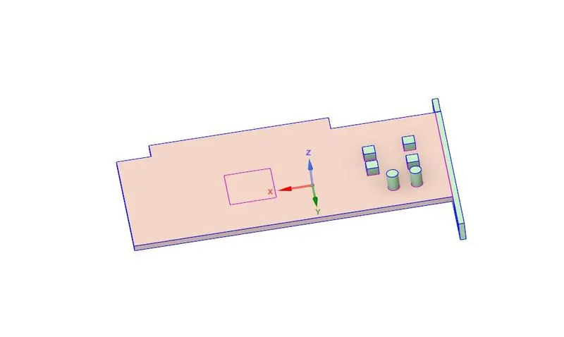
• A simplified model of graphics card is considered for this analysis. There are 3 distinct components in this model namely, the Base, Processor, and Fins.
• The base consists of everything except the fins and processor. It is assumed to be made of FR4(fire-resistant fiberglass).
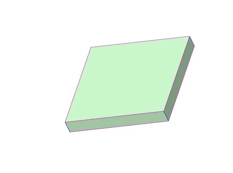
• The processor is assumed to be made of silicon. The electrical supply is given to the processor and it acts as a heat source during its working.
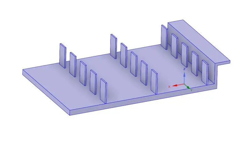
• The fins or extended surfaces are made up of aluminum and help in taking away the heat.
• Except for Aluminum, other materials are not present in the Fluent database. we need to create those materials for our analysis in Fluent.
• The processor is assumed to be powered with a 2 W supply. It's assumed that the entire power is converted into thermal energy. From a simple energy density equation, we can determine the thermal source term.
• The working fluid which flows in the enclosure for cooling purposes is air from the Fluent database.

PREPROCESSING:

Geometry

• Import the geometry to Spaceclaim.

• Base

• Processor

• FIns

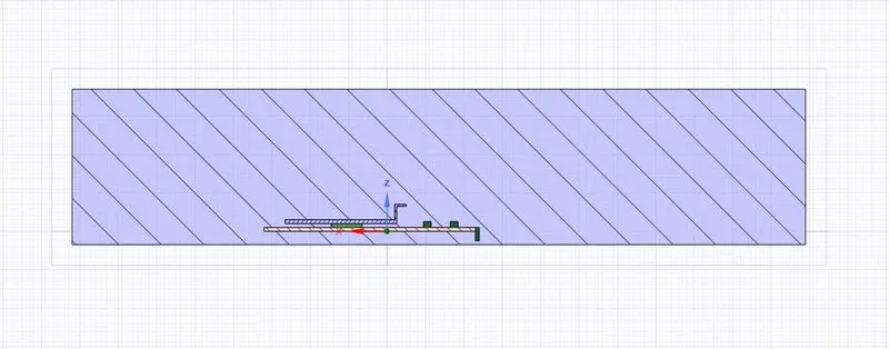
• Check whether the Share topology feature is turned on. We can verify it from a cut sectional view.

Meshing

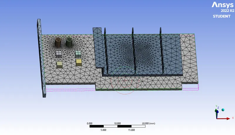
• In this analysis, we are performing simulations on different mesh sizes.
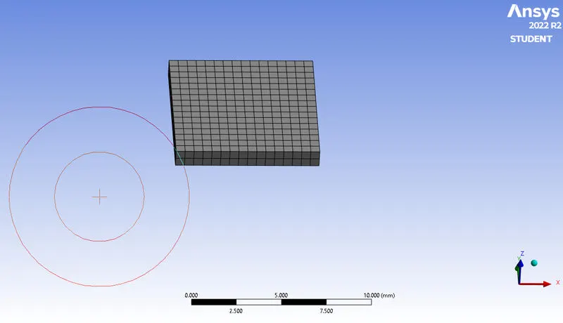
• Case 1 - (Total number of elements - 137618)

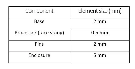
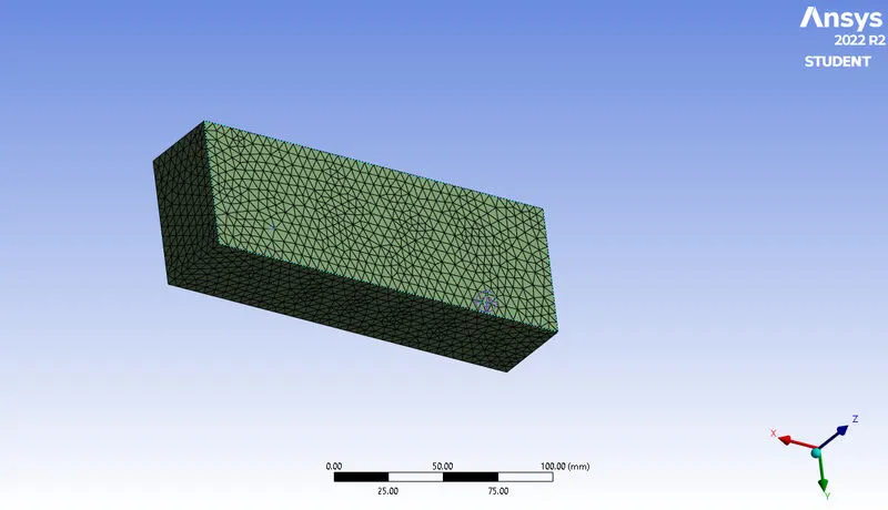
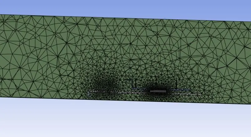
Base and Fins

Processor

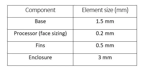
• Case 2 - (Total number of elements - 475272)

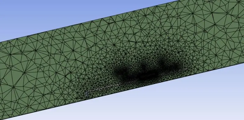
• Face sizing was done on the processor as the thickness is 1mm.
• The mesh element size was chosen in such a way that possible regions of hot spots get a refined mesh compared to the enclosure.
• The total number of mesh elements is limited to 500000. Therefore mesh refinement was done keeping that in mind.

Solvent setup

1.	Solver type	Pressure based
2.	Solver time	Steady-state
3.	Energy	On
4.	Turbulence model	k epsilon
5.	Material (Fluid)	Air
6.	Material (solid)	a) Aluminum b) Silicon c) FR4
7.	Inlet	Velocity inlet
8.	Outlet	Pressure outlet
9.	Method	Coupled

• Materials assigned for the simulation are as follows,

PART	MATERIAL	Thermal conductivity (W/mK)	Specific heat capacity (J/kgK)	Density (kg/m^3)
Fin	Aluminum	202.4	871	2719
Base	FR4	0.30	1100	1850
Processor	Silicon	153	703	2330
Fluid domain	Air	0.0242	1006.43	1.225

• As we discussed before, we need to assign a source term for the processor. The volume of the processor is 64mm^3 (8 x 8 x 1). If we assume that it generates 2 W of energy, we can calculate energy density as (2/64x10^-9) which gives us a value of 31250000 W/m^3.
• This value can be given under the Cell Zone Conditions tab.
• The simulation is run for 3 different values of velocities ie; 1m/s, 3m/s, and 5m/s for both Case 1 and Case 2.
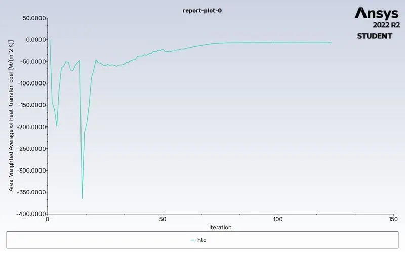
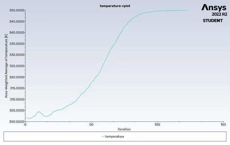
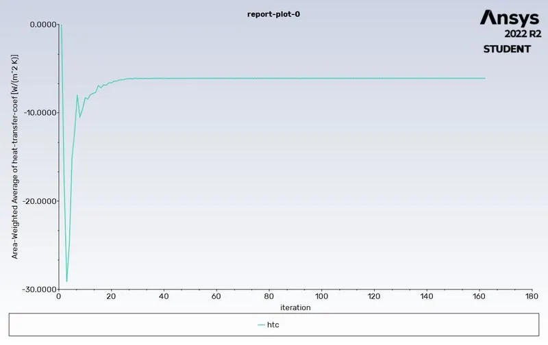
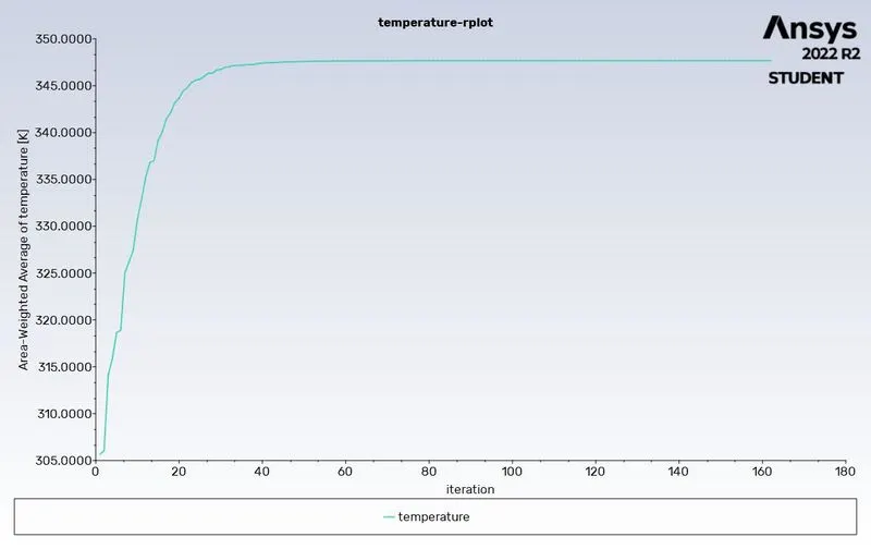
• Report definitions are created for the Surface heat transfer coefficient and temperature.
• Hybrid initialization is done and the simulation is run for 200 iterations.

RESULTS

Case 1

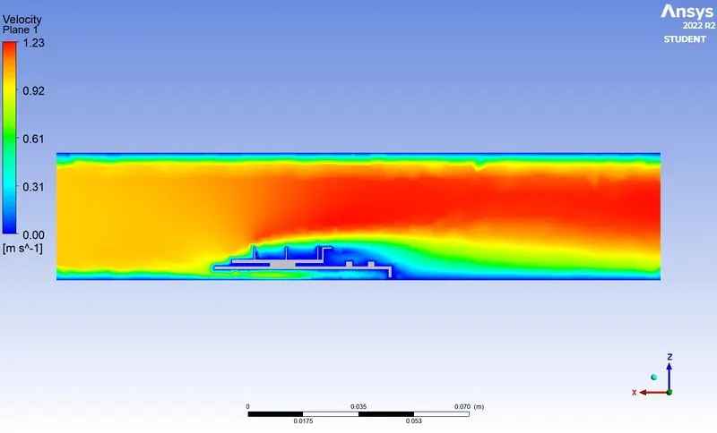
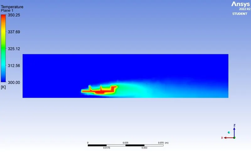
Inlet velocity - 1m/s

• Residuals

• Surface heat transfer coefficient

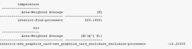
• Average temperature across the processor

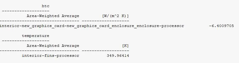
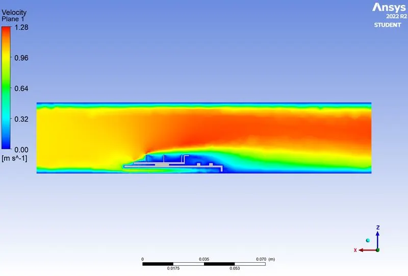
• Velocity contour across the graphics card

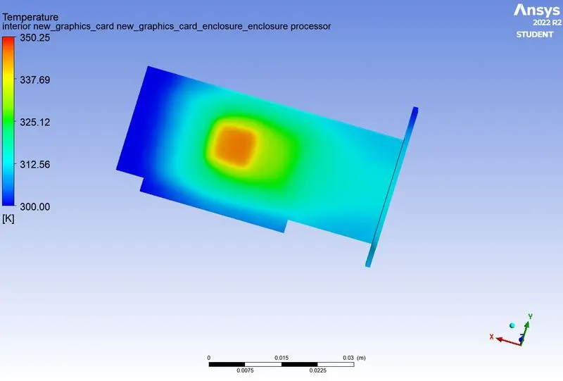
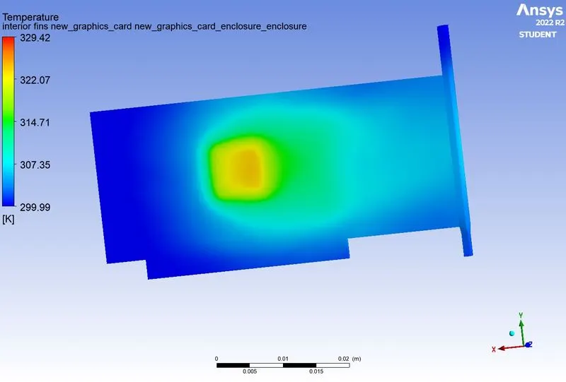
• Temperature contour

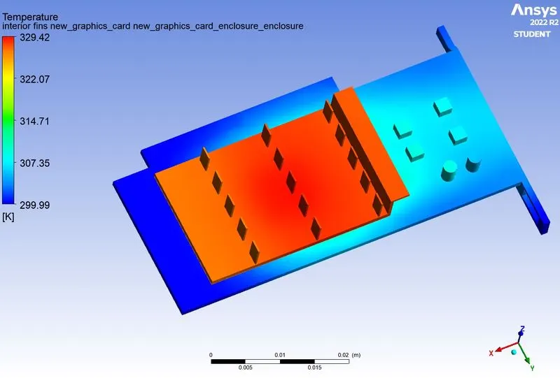
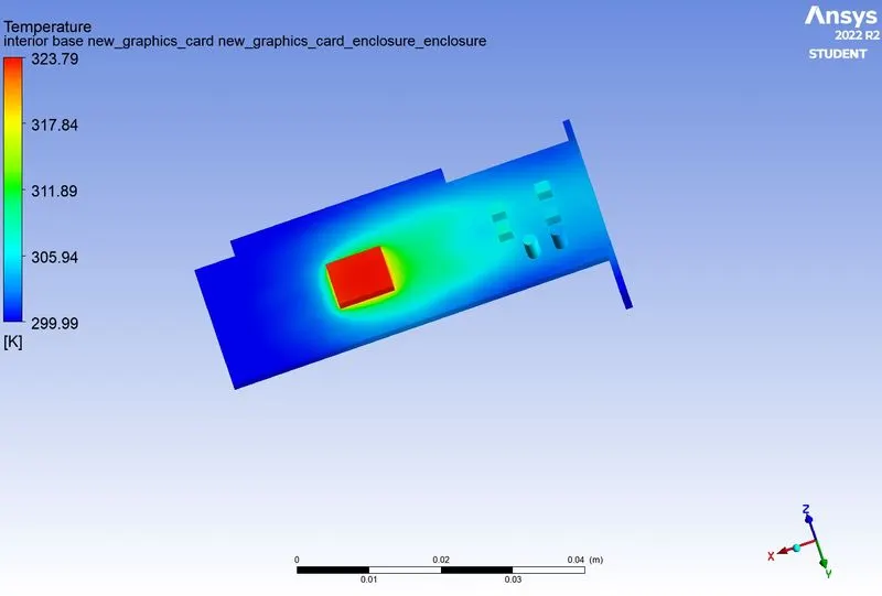
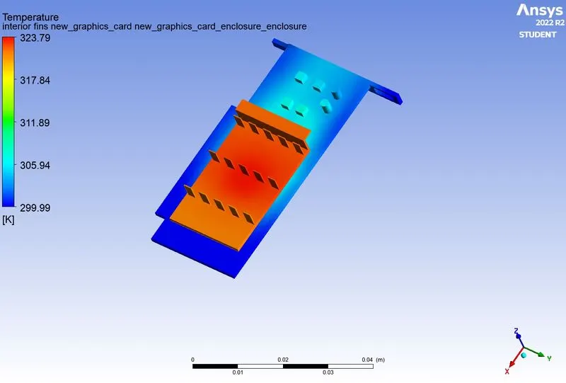
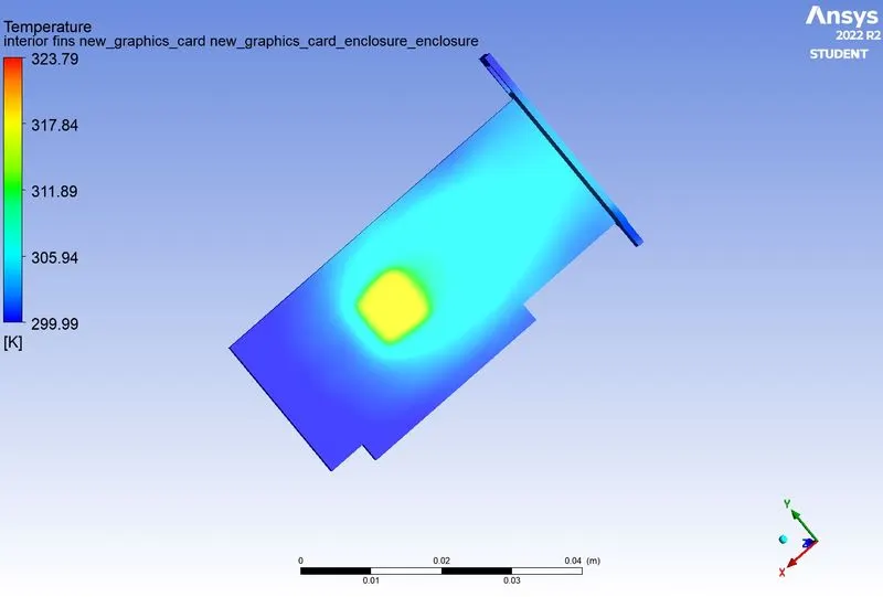
• Hotspots

Inlet velocity - 3 m/s

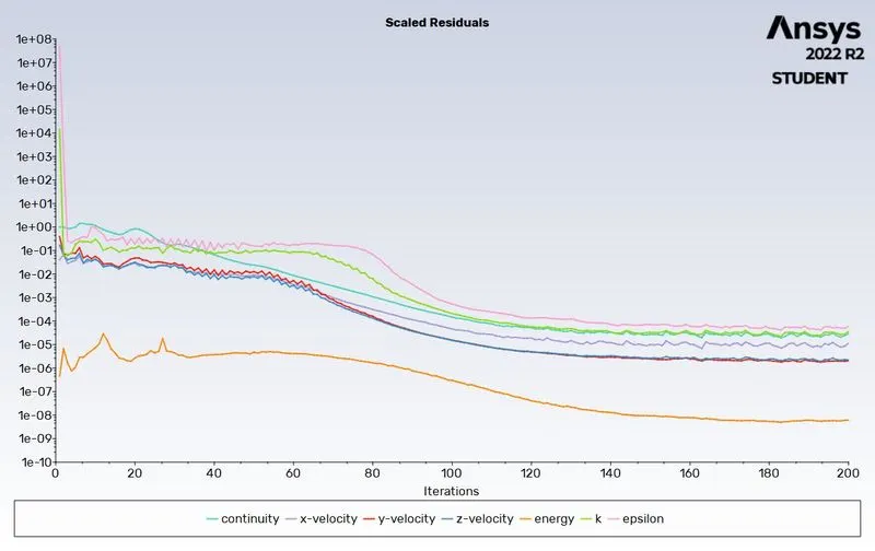
• Residuals

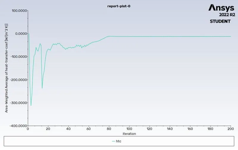
• Surface heat transfer coefficient

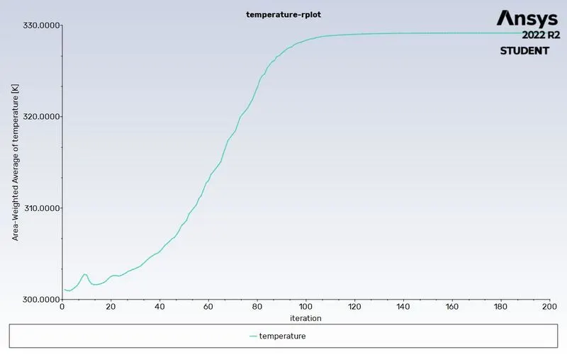
• Average temperature across the processor

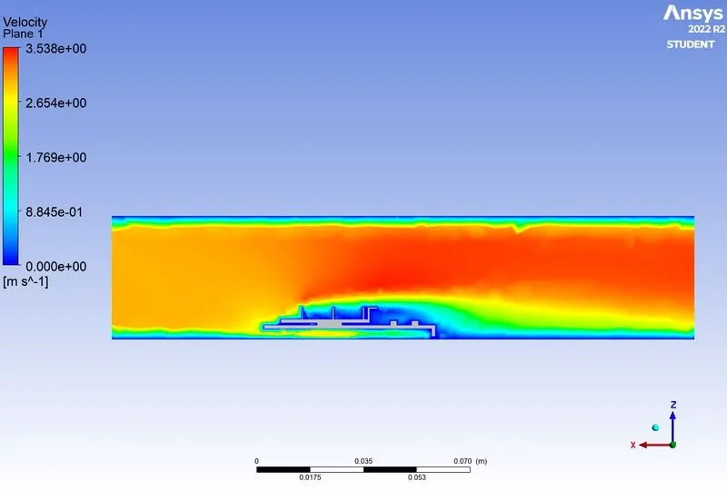
• Velocity contour across the graphics card

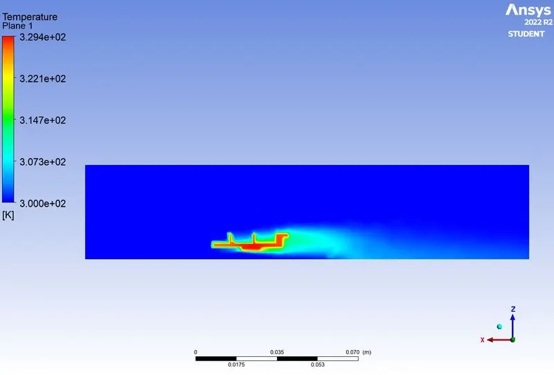
• Temperature contour

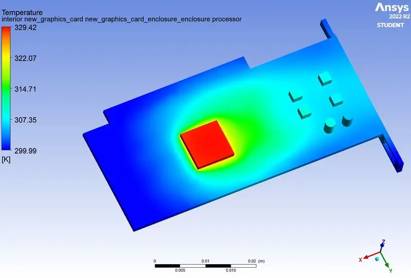
• Hotspots

Inlet velocity - 5 m/s

• Residuals

• Surface heat transfer coefficient

• Average temperature across the processor

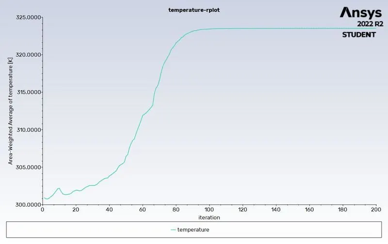
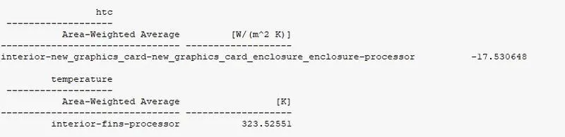
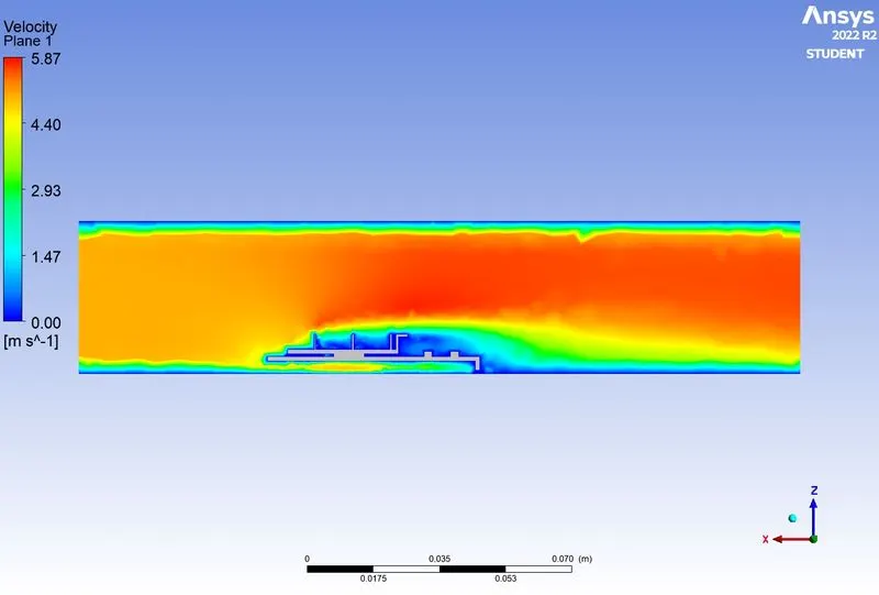
• Velocity contour across the graphics card

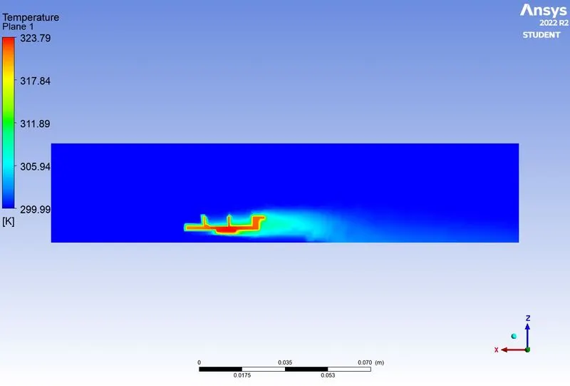
• Temperature contour

• Hotspots

Case 2

Inlet velocity - 1m/s

• Residuals

• Surface heat transfer coefficient

• Average temperature across the processor

• Velocity contour across the graphics card

• Temperature contour

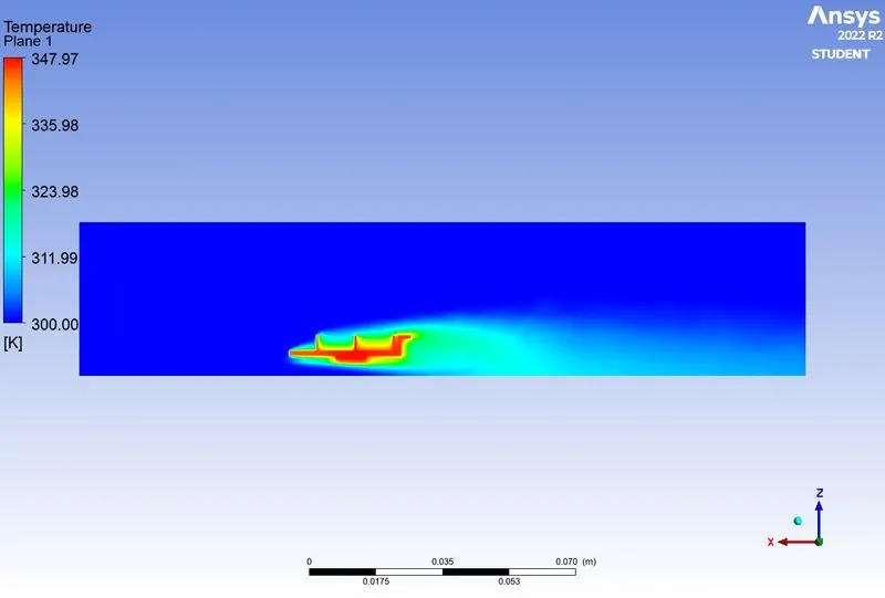
• Hotspots

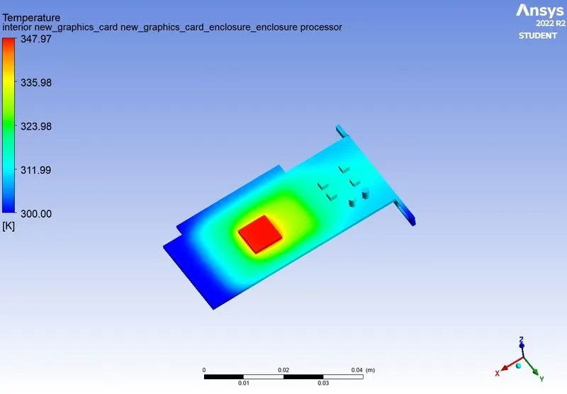
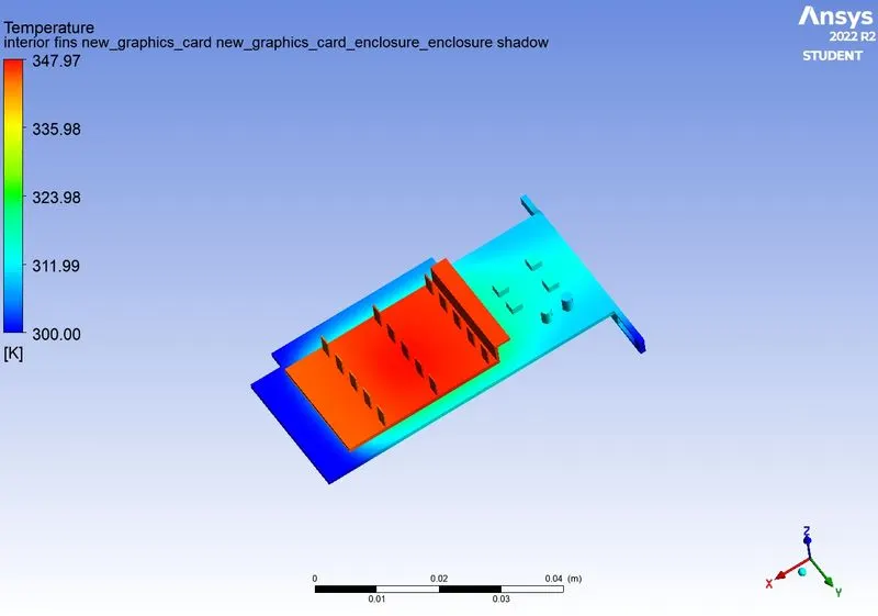
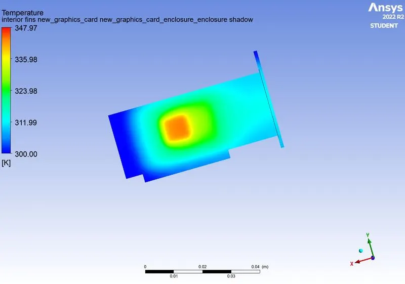
Inlet velocity - 3 m/s

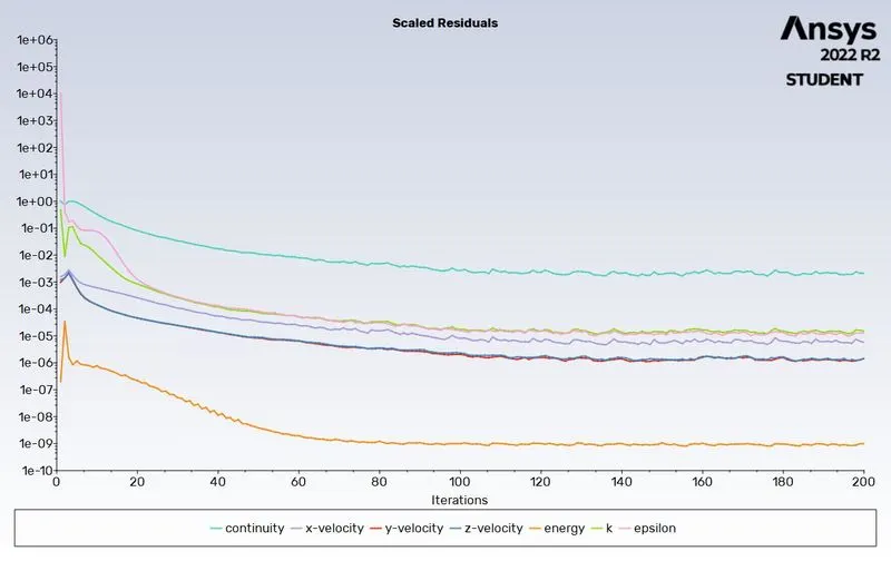
• Residuals

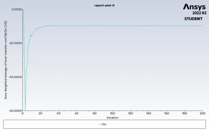
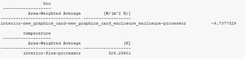
• Surface heat transfer coefficient

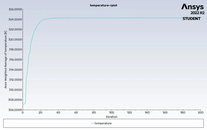
• Average temperature across the processor

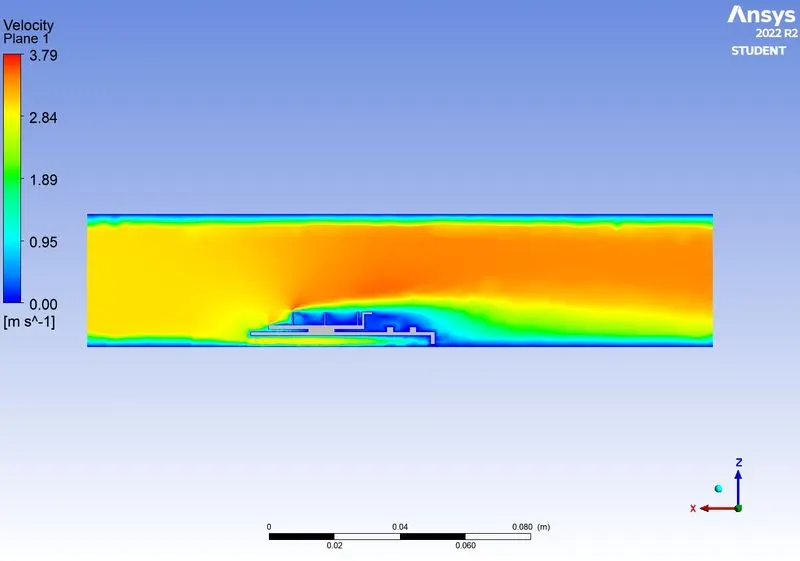
• Velocity contour across the graphics card

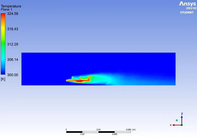
• Temperature contour

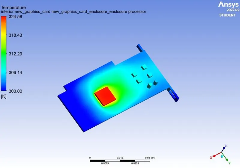
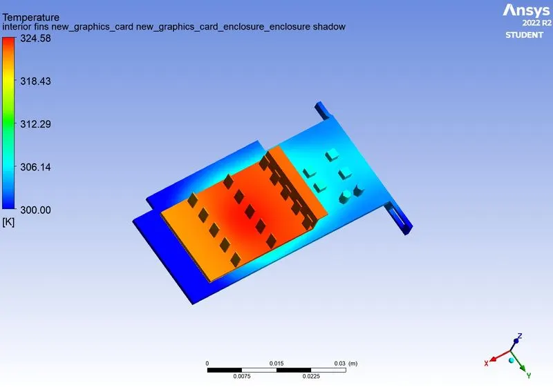
• Hotspots

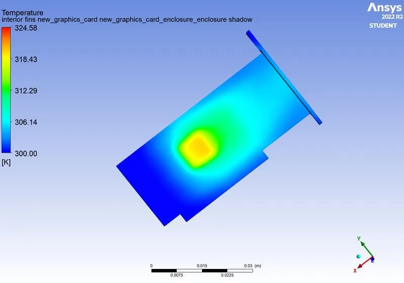
Inlet velocity - 5 m/s

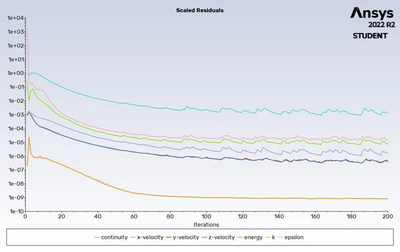
• Residuals

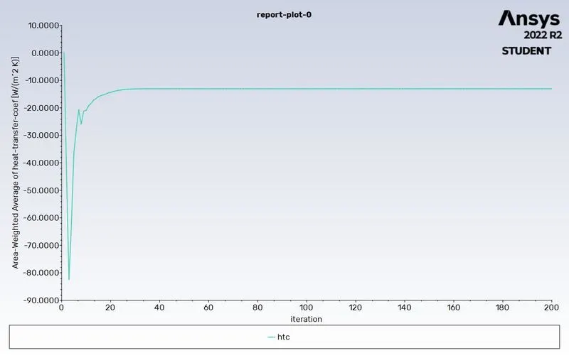
• Surface heat transfer coefficient

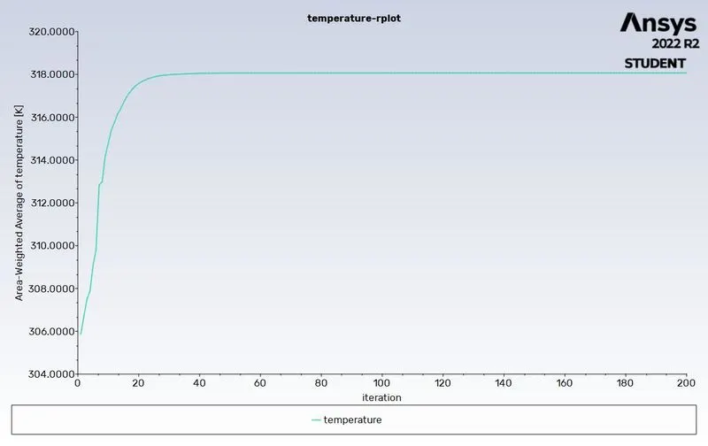
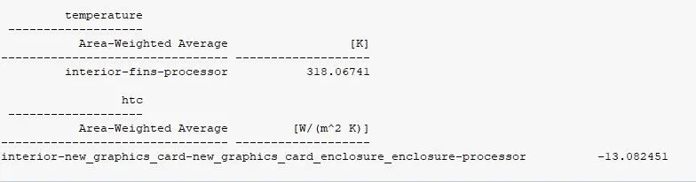
• Average temperature across the processor

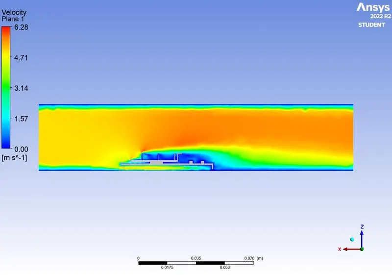
• Velocity contour across the graphics card

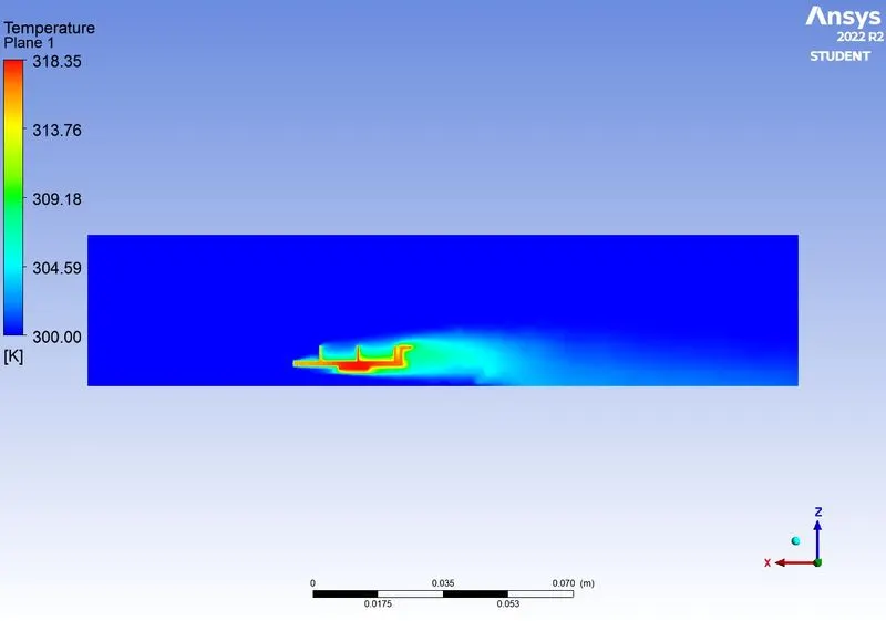
• Temperature contour

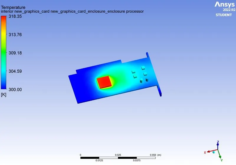
• Hotspots

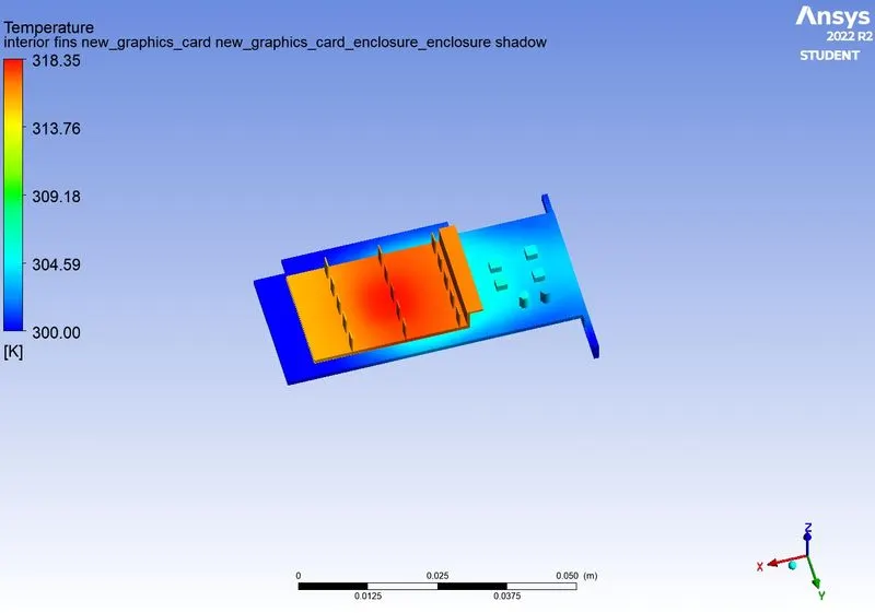
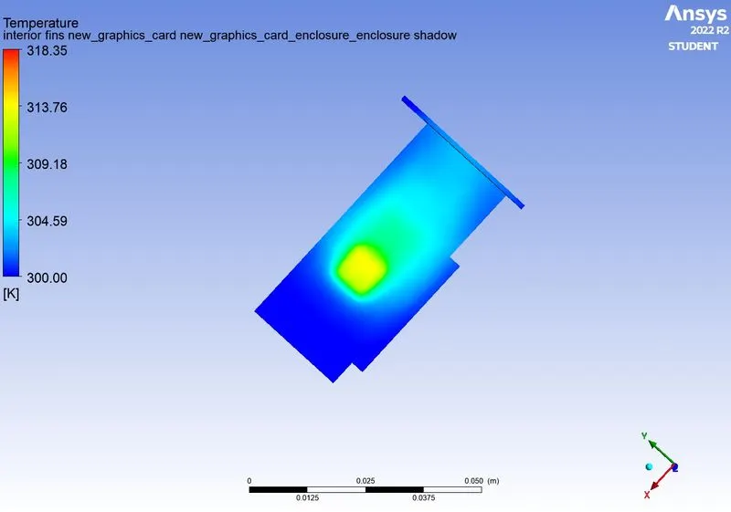
• Comparison chart

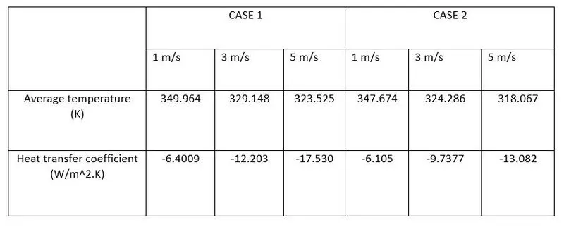
CONCLUSIONS:

1. From the above table, we can see that the average temperature decreases as we increase the inlet air velocity.
2. The heat transfer coefficient is highest for the inlet velocity of 5m/s. This observation is in line with the experimental trend.
3. Thermal hotspots can be observed near the fin-processor interface and the fin body.
4. From the residual plot, we can infer that the solution has converged.
5. Providing mesh refinement for processor and fins gave results closer to experimental values.