Week 6 - CHT Analysis on a Graphics card

Aim:

To Perform a steady-state conjugate heat transfer analysis on a model of a graphics card. You can use appropriate materials of your choice for the simulation. Make sure to properly define the correct solid and fluid zones. Refer the video for further clarification and the model is provided below the video.

Run the simulation for best possible mesh with combination of coarse and refined mesh in different regions. Explain the reason for choosing the particular mesh settings.

Objectives:

In this challenge they are give some objectives so we have to follow as.

1. Run the simulation by varying the velocity from 1m/sec to 5m/sec for at least 3 velocities and discuss the results.
2. Find out the maximum temperature and heat transfer coefficient attained by the processor.
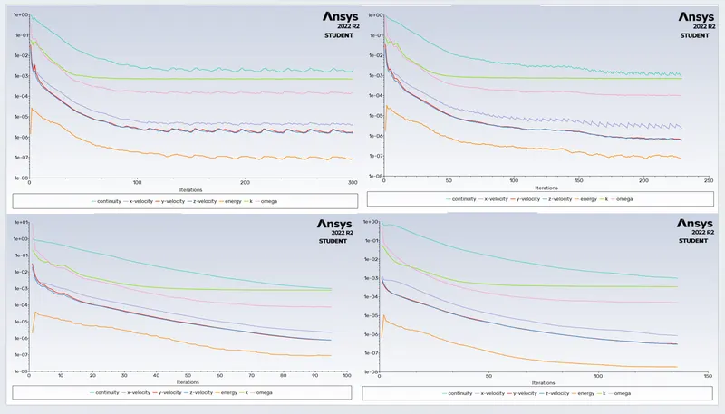
3. Prove that the simulation has achieved convergence with appropriate images and plots.
4. Identify potential hotspots on the model.

CHT Analysis:

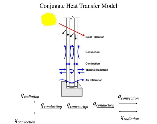
Conjugate heat transfer corresponds with the combination of heat transfer in solids and heat transfer in fluids. In solids, conduction often dominates whereas in fluids, convection usually dominates. Conjugate heat transfer is observed in many situations.

Conjugate Heat Transfer Analysis. The analysis type Conjugate heat transfer (CHT) allows for the simulation of heat transfer between Solid and Fluid domains by exchanging thermal energy at the interfaces between them. Typical applications of this analysis type exist as, but are not limited to, the simulation of heat exchangers, cooling of electronic equipment, and general-purpose cooling and heating systems.

Graphics Card:

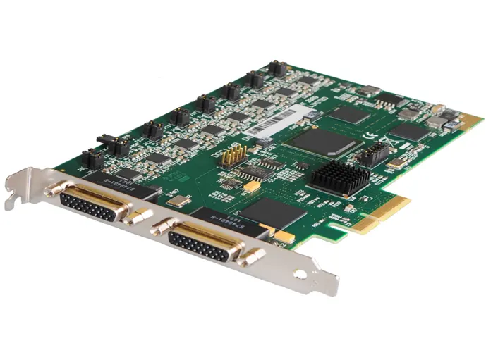
A Basic Definition of Graphics Cards GPU stands for graphics processing unit. You’ll also see GPUs commonly referred to as graphics cards or video cards. Every PC uses a GPU to render images, video and 2D or 3D animations for display. A GPU performs quick math calculations and frees up the CPU to do other things.

Graphics card is a hardware which is used to increase the video memory of a computer, and make its display quality more high-definition. It makes the computer more powerful and gives it the capacity to do more high-level works. The quality of the image depends on the quality of the graphics card.

Challenge Approach:

In this challenge we have to solve 4 cases by using ANSYS Fluent solver. We will be using ANSYS Fluent solver to create the geometry and perform structured tetra CFD mesh, setup the physics of fluid flow and run the iterations to get solutions, using post processing we will get the plots, contours, vectors, streamlines etc.,

In this challenge we have to use velocity 5m/s and k-omega SST model we shall study grid independence for CHT analysis study. When we say grid independence study, we shall study for 4 cases as follows,

Cases Flow domain Body element size (mm) velocity

element size (mm)

Case 1 10.29 10.29 5

Case 2 10.29 10.29 3

Case 3 10.29 10.29 1

Case 4 10 1 5

As usual in this challenge also using five major steps those are geometry, meshing, set-up, solution and results.

Step 1: Geometry

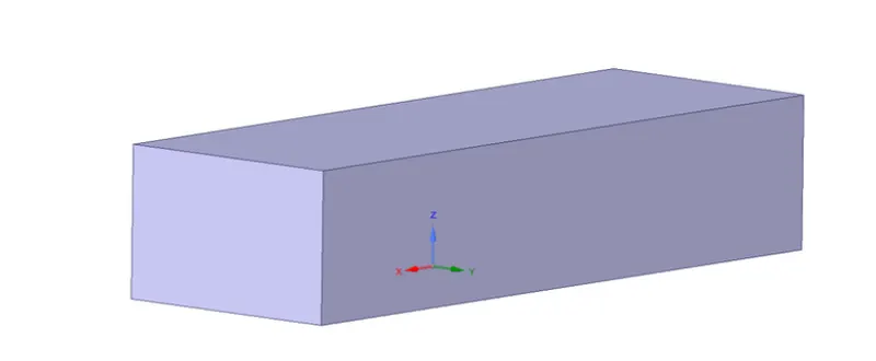
First step is we have to upload the given geometry file in ansys fluent workbentch. After that we have give share topology. In this challenge only one step is enough for this geometry. Once we completed the geometry after that we can able to move next meshing process.

Step 2: Meshing

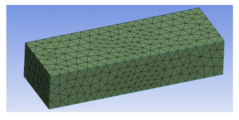
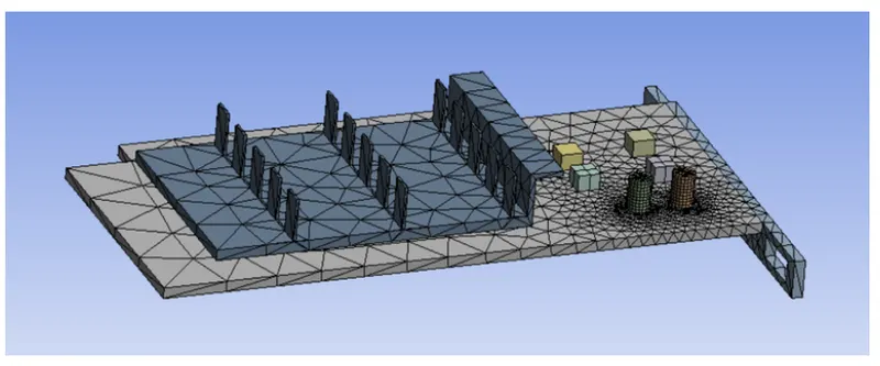
In this challenge the step 2 is meshing process so we can right click and open the Mesh. In the mesh tab the geometry is already preloaded for meshing process so we have to click the GENERATE MESH option it should create a mesh automatically. In this process we have to give 10.29 mm element size, in this challenge three cases the element size is same. In this challenge we have to change the fourth case only the element size 10mm for flow domain and 1mm for body mesh size. Once we done this meshing process, we can see the green tick symbol nearby Mesh option. So, we can able to move the next set-up process.

Step 3: Set-up

In this challenge the 3rd process is set-up process so we have to right click and open the Setup tab. In the Fluent launcher select 3D, double precision and select the number of cores as per the user system configuration and click on start. Upon opening, there are some selections to be done to define the simulation definitions. In the set-up process we can able to select the Type: Pressure based, Velocity Formulation: Absolute, Time: Steady.

Next, we go to physics tab, we can turn on energy and then we can turn on viscous and select k-omega > SST as well.

Under the materials we shall select air as our default material with material type as fluid. since we are dealing with the CHT analysis, we shall consider the solid volume also with aluminium as the default solid material. We need to add 2 more materials for Processor and the PCB which can be done by copying the aluminium and changing the properties like density, specific heat and thermal conductivity from standard data books for materials as follows, the name of the materials is polystrene, siliicon.

Body Material Thermal conductivity (W/m.K) Specific heat (J/Kg.K) Density (Kg/m^3)

Fins Aluminium 202.4 871 2719

Processor Silicon 153 703 2330

PCB Polystyrene 0.027 1210 55

Flow domain Air 0.0242 1006.43 1.225

In the cell zone conditions, select the solid volume and check for material selection is solid, and fluid material for fluid volume. For processor after selecting the material, enable source term and input 31250000 W.

Q = 2 W, Qg = Q/V

V = 8*8*1 e-9

Qg = 2/64 = 31250000 W/m^3

We can proceed to define boundary conditions, as follows

Inlet: velocity magnitude = 5 m/s

Outlet should be a pressure outlet

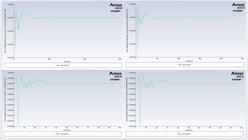
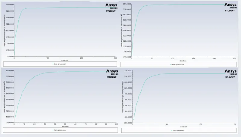
If we want to create the surface reports, we have to click on the Solution > Reports > Definitions > New > Surface Report > Area weighted average > Wall fluxes > Surface heat transfer coefficient for the heat transfer coefficient in the processor. And create another report for the temperature of the processor also. In order to start the simulation for the above set up physics, we need to initialize the entire flow field by clicking on the t=0 initialize icon. In the Run Calculation we can input the number of iterations to be run in this case 300 and clicking on the Calculate should start the iterations.

Once we complete the iterations calculation, we can get the scaled residuals, average temperature plot and surface heat transfer plot. We need temperature contour as well, to get them Results > Graphics > Contours > New temperature for temperature contour. Once we completed the set-up option after that we can able to move next solution process.

Step 4: Solution

Some solutions are calculated in set-up option itself. So almost completes the solution process also so we can able to move next process of the results option.

Step 5: Result

In this challenge we are going to see the final step of result so we have to right click it is also called Post processor. The result tab default view is a wireframe model, we can create a plane in XZ to view contours by using location option. The solution, all contours and plots can be created here. In this challenge for Case 4, we shall repeat the same. We can simply right click and select DUPLICATE option get duplicate same procedure we have to follow for 2, 3, and 4 cases also. In that set-up process for under materials we shall input same material for 4 cases but the meshing only is different for case 4 and then we can change the velocity for 4 cases then completed the result process also. Finally, we completed the all steps.

Result temperature plots contors and vectors images:

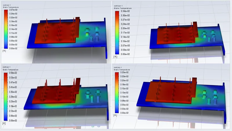
Four cases temperature with fin contours:

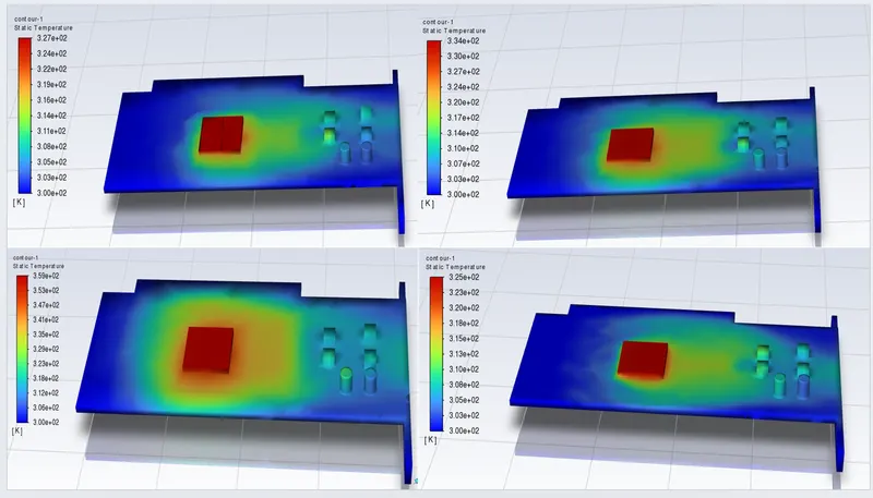
Four cases temperature without fin contours:

Four cases residuals plot:

Four cases SHT plot:

Four cases tem-processor plot:

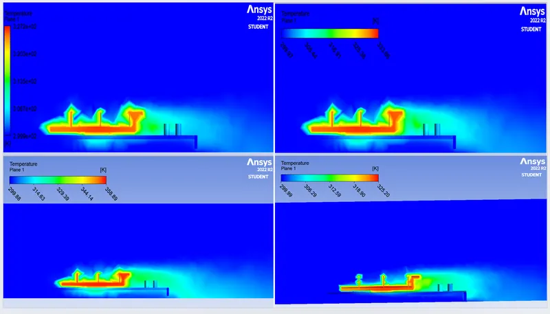
Four cases temperature contour:

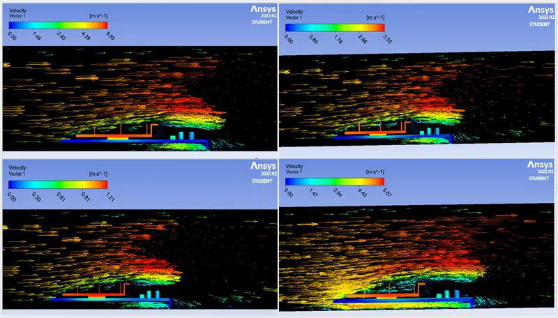
Four cases velocity vector contour:

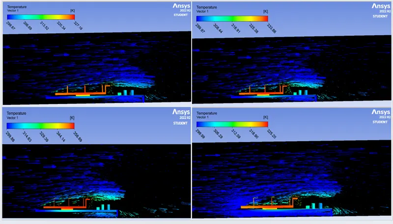
Four cases temperature vector contour:

CONCLUSION:

Finally, we get the results for 4 cases, let us tabulate for surface heat transfer coefficient and maximum temperature of processor with respective grid sizes, velocities.

Case 1 Case 2 Case 3 Case 4

Flow domain mesh (mm) 10.29 10.29 10.29 10

Body mesh (mm) 10.29 10.29 10.29 1

No.of elements 83397 83397 83397 166592

Surface heat transfer coefficient (W/m^2.K) 1.57 6.059 2.65 7.121

Maximum temperature of processor (K) 327.2 333 358.8 325.3

Inferences:

In this challenge I observed the finer size mesh elements doesn’t affect the surface heat transfer coefficient much, when compare the four cases the third and fourth cases are easily converged whereas the maximum temperature attained by the processor is lower in case of the finer mesh. This area of heat affected in PCB is visible in Temperature contour without fins, where at low velocities the heat affected area is large. Hence, we need a good inlet velocity to maintain the temperature of processor, in this case 5 m/s velocity is give better result.

References:

https://www.geeksforgeeks.org/what-is-a-graphics-card/

https://www.researchgate.net/publication/327775953_Modeling_of_Conjugate_Heat_Transfer