Week 6 - CHT Analysis on a Graphics card

OBJECTIVE:

• The objective of this project is to perform a steady state conjugate heat transfer (CHT) analysis on a graphics card.
• To run the simulation by varying the velocity 1m/sec 3m/sec 5m/sec.
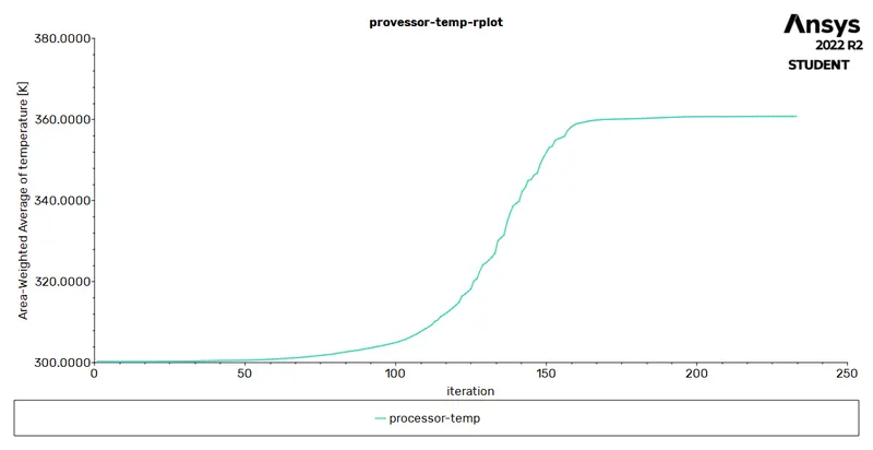
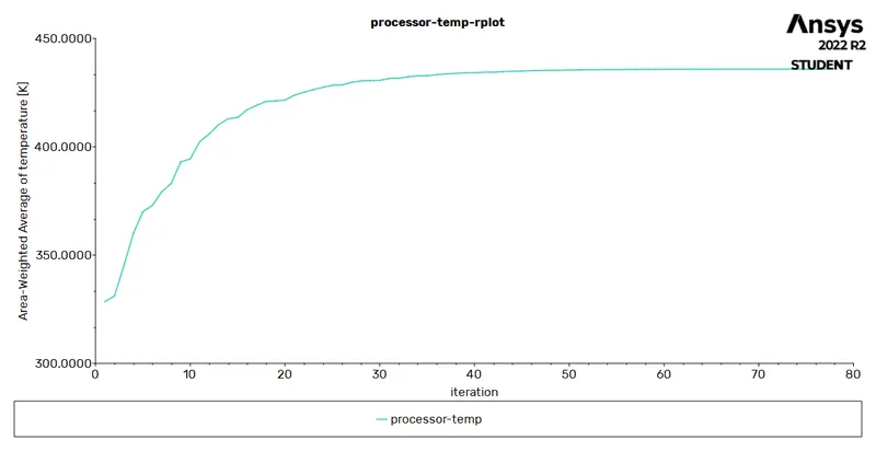
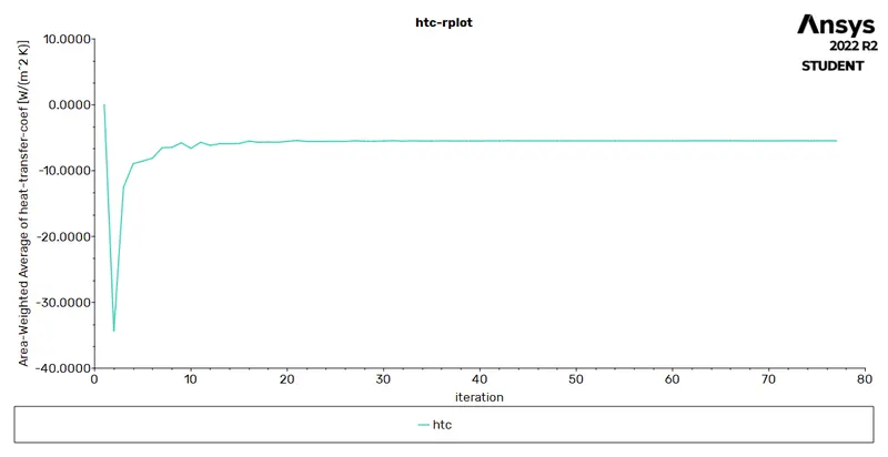
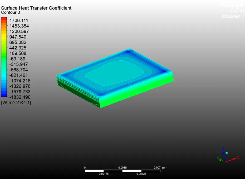
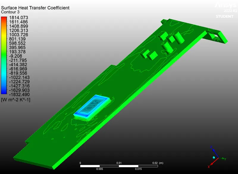
• To find out the maximum temperature and heat transfer coefficient attained by the processor.
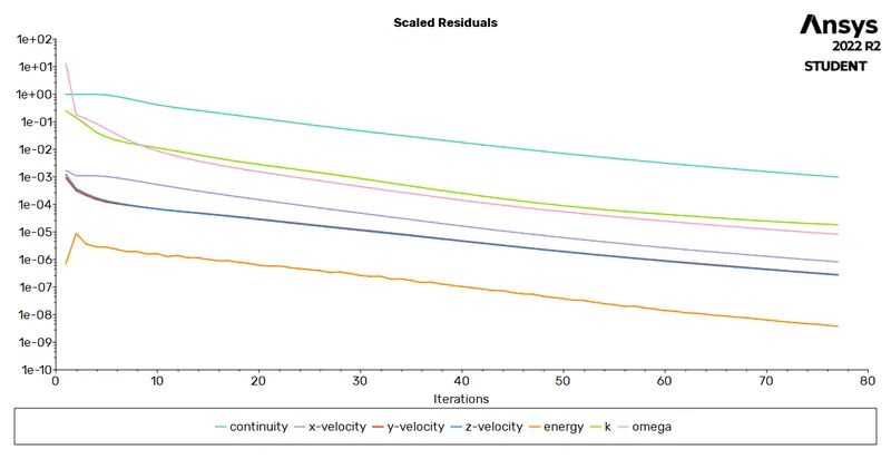
• To prove that the simulation has achieved convergence with appropriate images and plots.
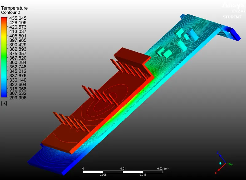
• To identify potential hotspots on the model.

Conjugate heat transfer (CHT):

Conjugate heat transfer is a type of heat transfer analysis between solids and fluids. This type of heat transfer includes both convective (between fluids) and conductive (between solids) heat transfer, as well as both forced and natural convection.

Modelling Procedure:

1: Pre-Processing.

• Open Ansys Workbench→under Analysis system select Fluid flow(fluent) drag and drop it in Project schematic → Geometry → New spaceclaim geometry.
• File select the appropriate file and then Open the file.
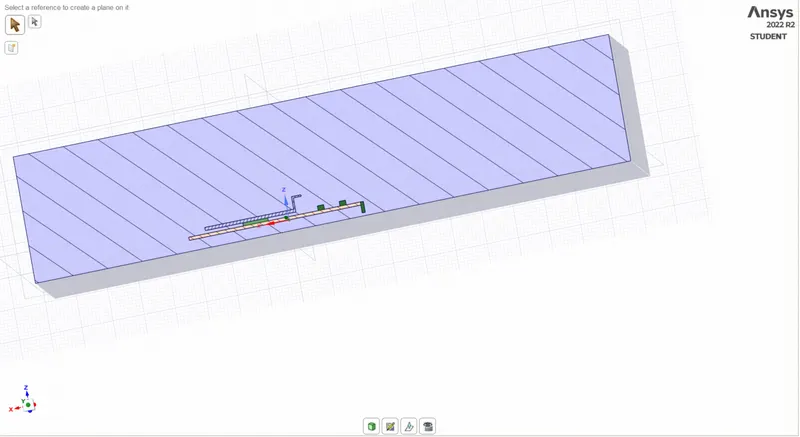
• Since we have defined an enclosure volume and the model has many components, we need to share the nodes between these two bodies which will be created while meshing, to share the nodes we are using Share topology option.

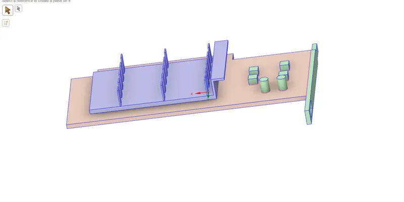
Graphic Card:

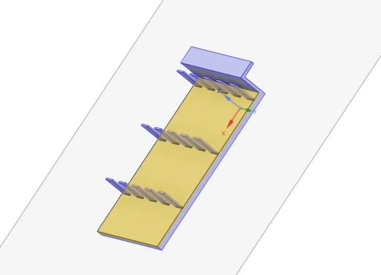
Fins:

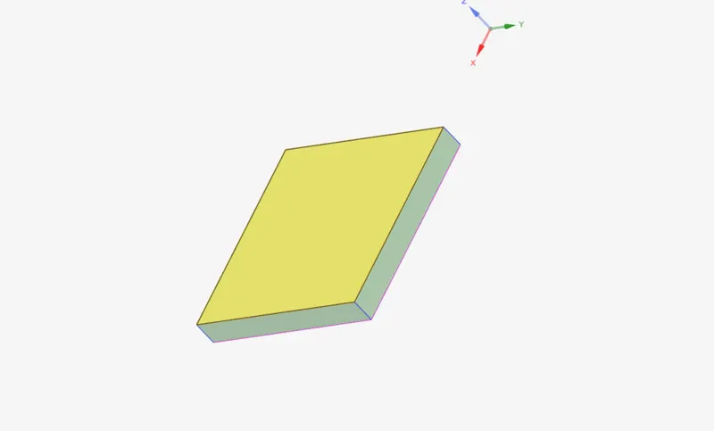
Processor:

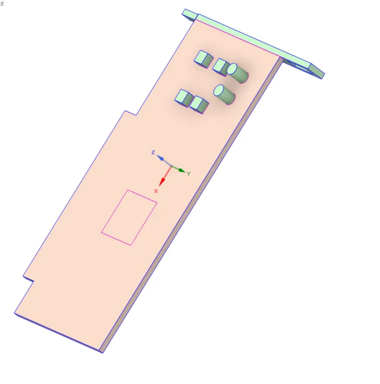
Base:

Shared Topology:

2: Meshing.

• Before generating a base mesh, let's name the different components of the graphic card so it is easier to find them while setting up fluent.
• We will proceed with mesh generation for required mesh element length using the Sizing and Inflation options. Mesh → Details of “Mesh” → Element Size then specify the required mesh length.
• Base, processor and fins are basic name selections which will help us in the simulation.
• Click generate mesh to create a base mesh, body sizing can be applied for the 3 solid components.

Base Mesh:

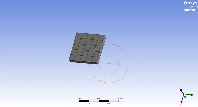
1:Processor:1.5mm.

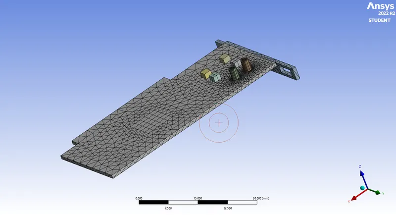
2:Base:2mm.

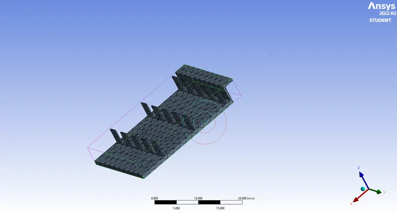
3:Fins:2mm.

4:Enclosure:5mm.

Processor:

Base:

Fins:

Enclosure:

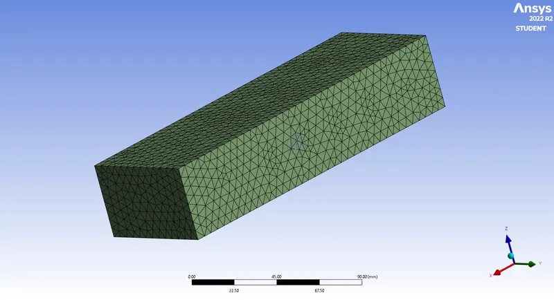
Mesh Quality:

No. Of elements= 101874.

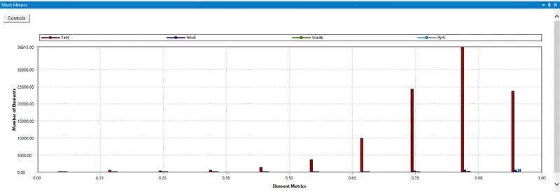
Refined Mesh:

1. Processor: 0.5mm.
2. Base: 0.75mm.
3. Fins: 0.75mm.
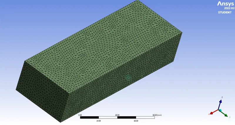
4. Enclosure: 3mm.
   

Processor:

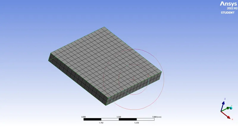
Base:

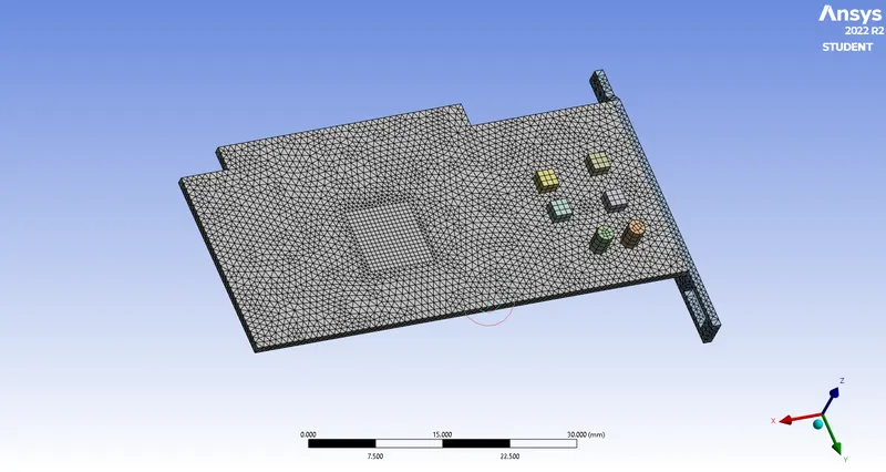
Fins:

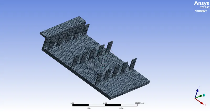
Enclosure:

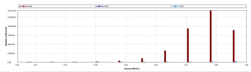
Mesh Quality:

No. Of elements: 371968.

3: Simulation.

• Setting up for Physics. Choose pressure-based solver and steady state condition.
• Since we will be studying heat transfer, we should enable Energy equation option.
• The turbulence model we are using is K-omega turbulence model.
• Then we have to define materials for different components under Materials. Then we have to assign the materials to the parts under Cell Zones.

Properties of Selected Materials:

Parts	Materials	Thermal Conductivity (W/mk)	Specific Heat Capacity (J/kg.k)	Density (kg/m^3)
Fins	Aluminium	202.4	871	2719
Base	FR-4	0.25	1300	1250
Processor	Silicon	153	703	2330
Heat transfer Fluid	Air	0.0242	1006.43	1.225

FR-4

FR-4 is a glass-reinforced epoxy resin laminate that stands for “Flame retardant”. it has a high working temperature, good heat resistance, good moisture resistance, good hole metallization performance. Therefore, it is preferred to build PCB.

In this project, the base plate is considered as a circuit board so FR-4 material was used for it.

FR-4 material is not present in fluent therefore it was created, for this simulation, using user define material by changing the name and properties of the existing material.

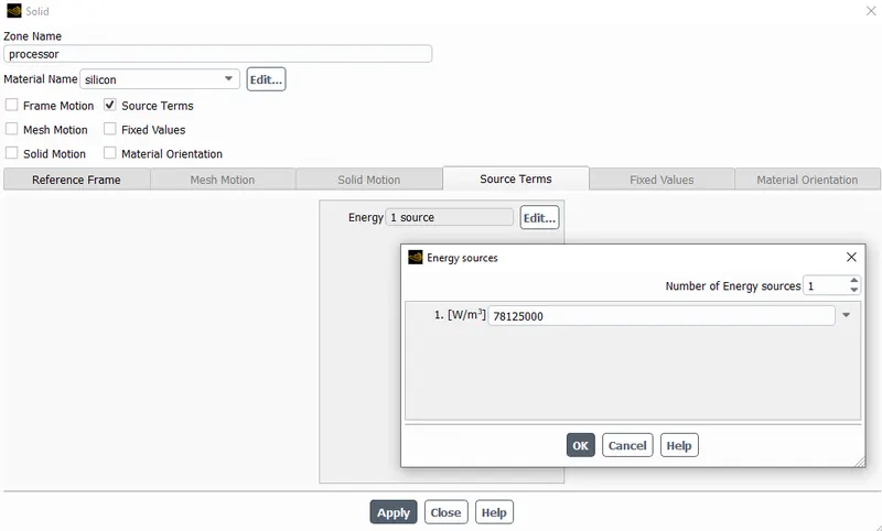
• Our main source of heat is the processor, so we have to define it as heat source and provide the heat generated value.

The heat generated by the processor:

Assuming the Card Power=5w.

Volume of the processor=64m^3.

Energy produced by the processor=5/64x10^-9.=78125000w/m^3.

Base Mesh:

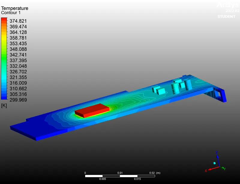
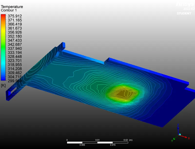
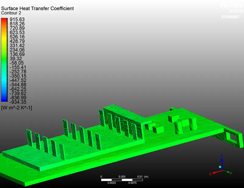
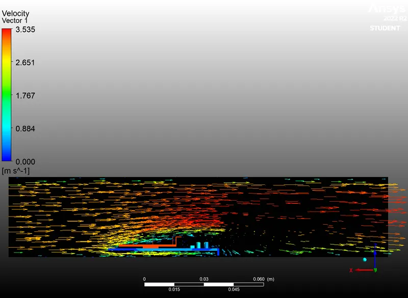
Inlet velocity=3m/s.

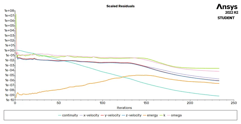
Scaled Residual:

Processor-temperature:

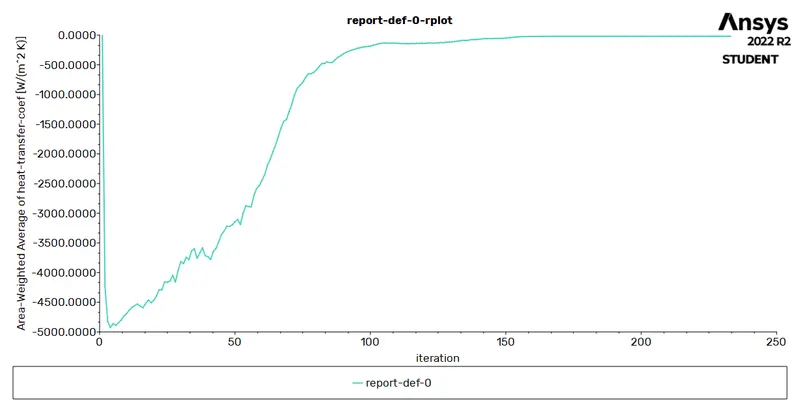
Heat transfer coefficient:

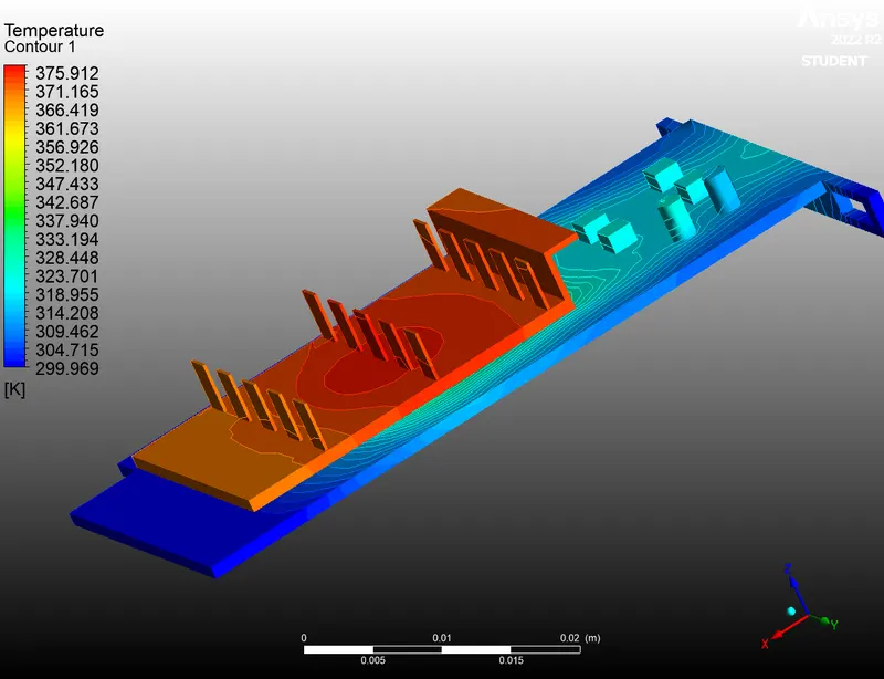
Temperature Contour:

Heat transfer coefficient:

Velocity Vector:

Refined Mesh:

Case1: Velocity inlet=1m/s.

Scaled Residual:

Processor Temperature:

Heat Transfer Coefficient:

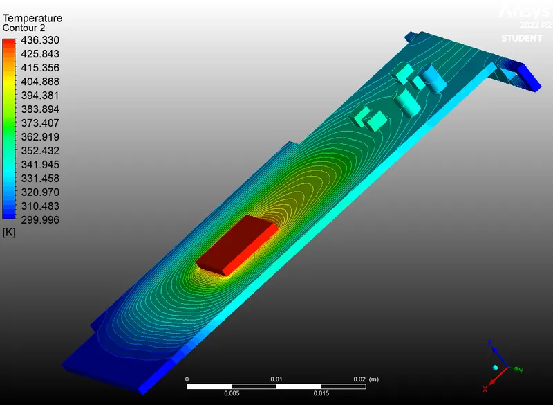
Temperature Contour:

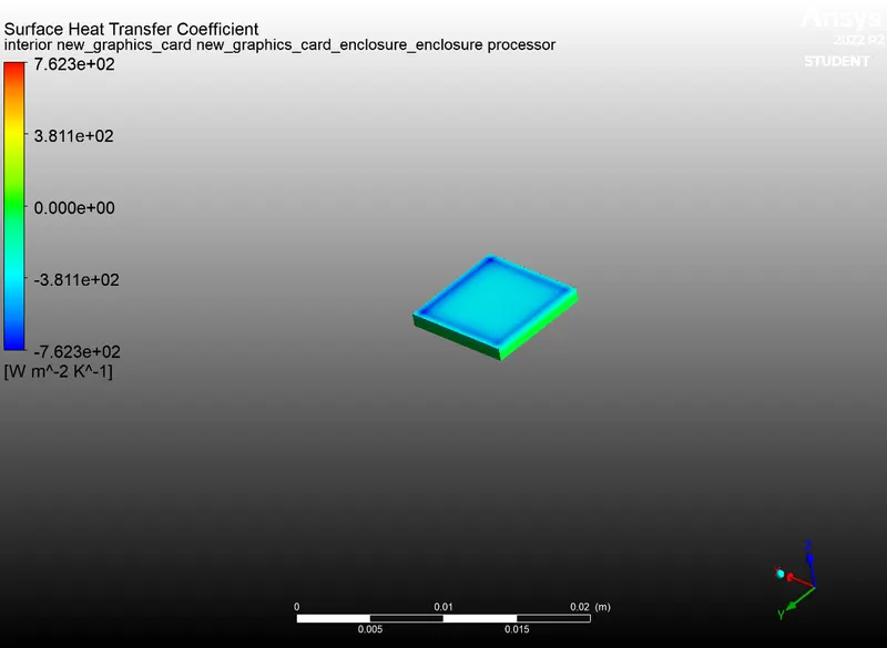
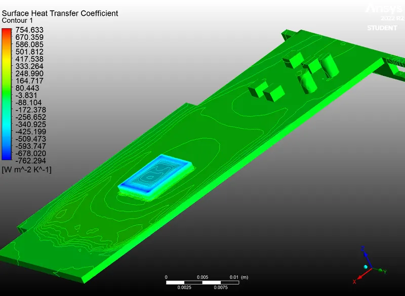
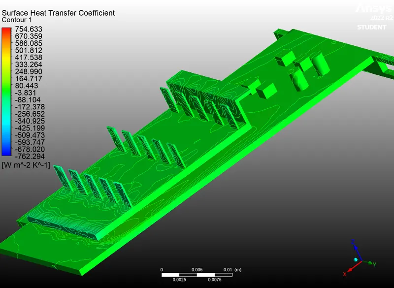
Heat transfer coefficient:

Velocity Vector:

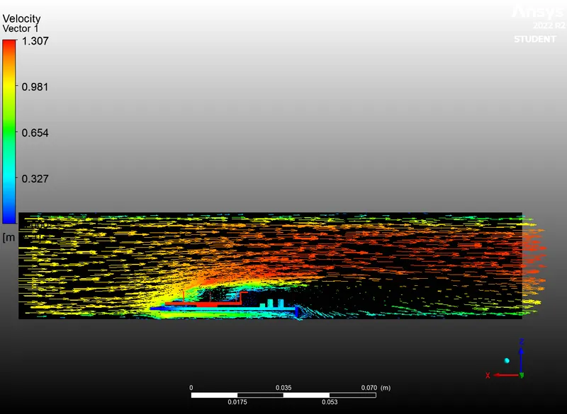
Case2: Velocity inlet=3m/s.

Scaled Residual:

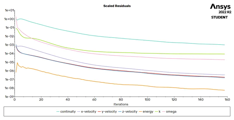
Processor Temperature:

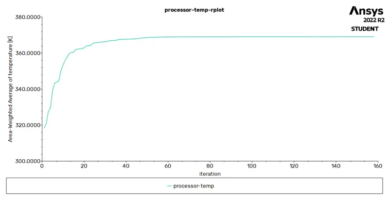
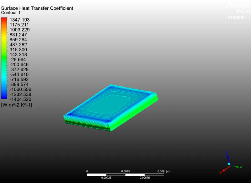
Heat Transfer Coefficient:

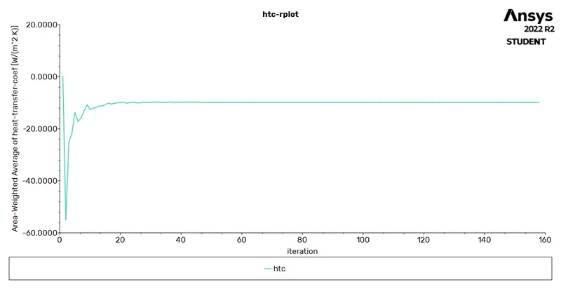
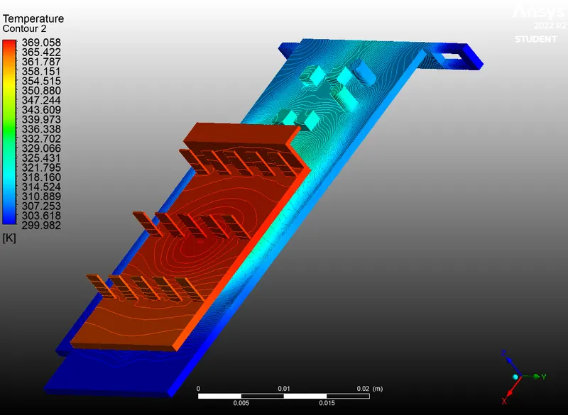
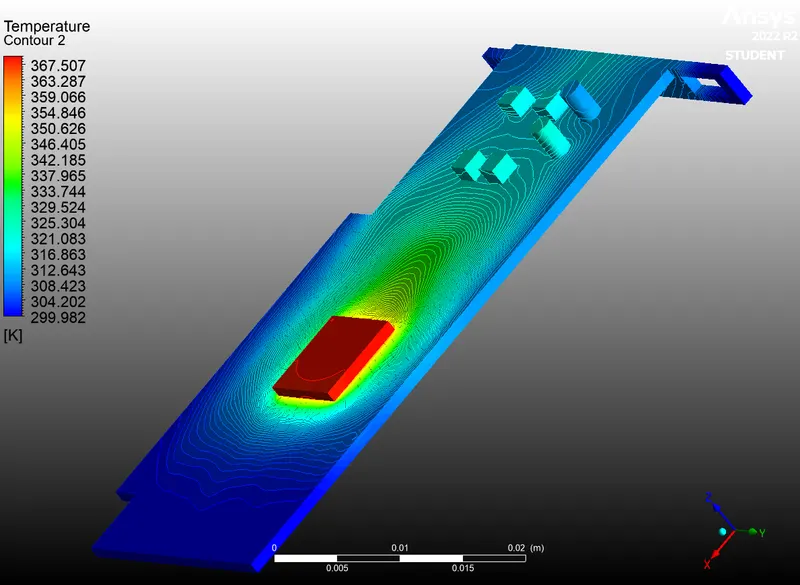
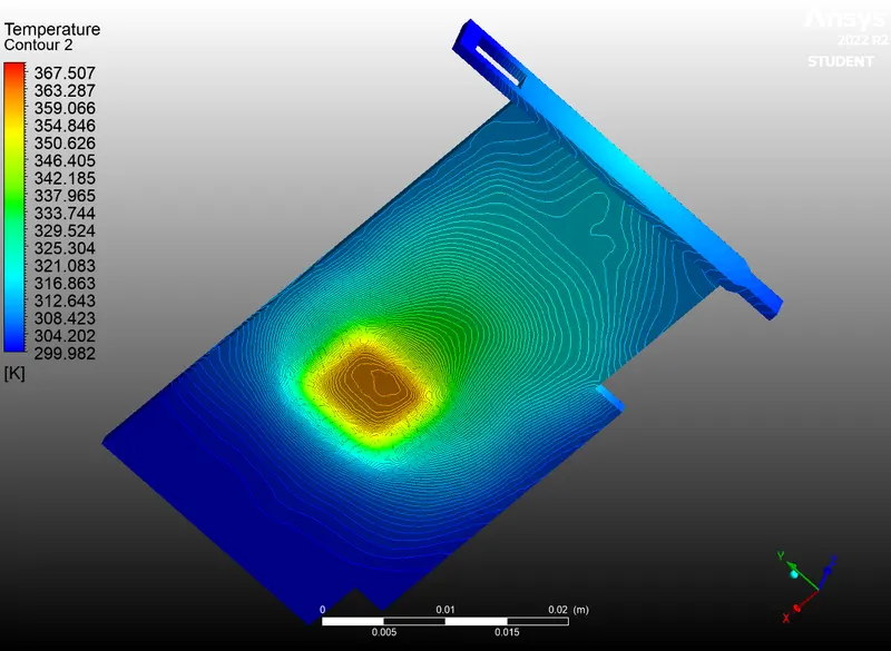
Temperature Contour:

Heat transfer coefficient:

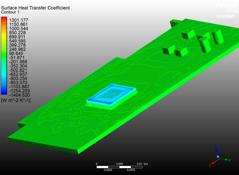
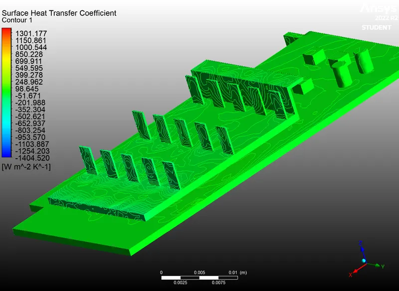
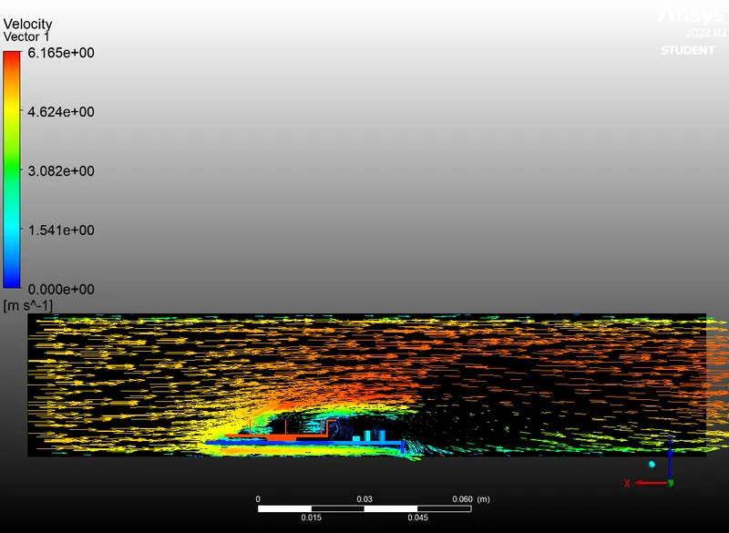
Velocity Vector:

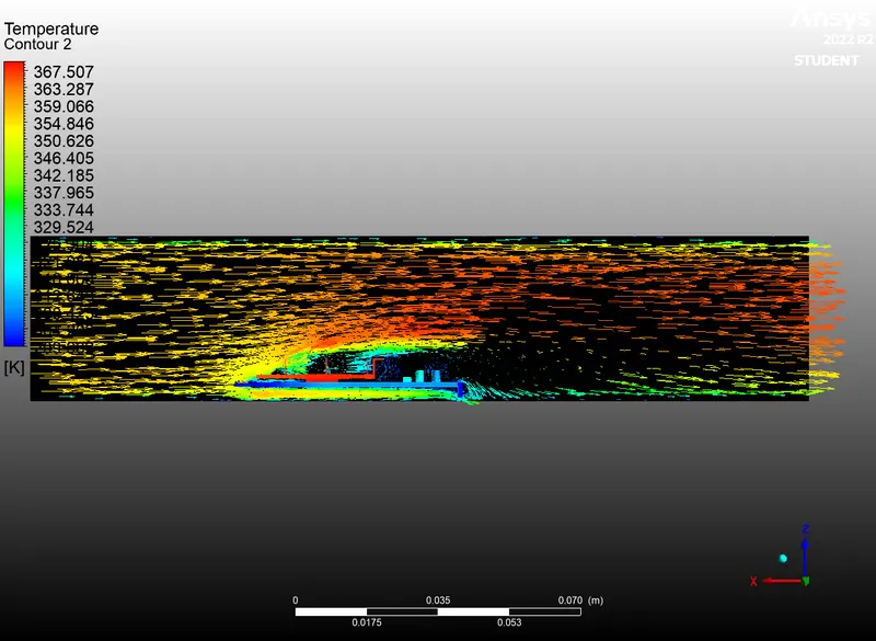
Case3: Velocity inlet=5m/s.

Scaled Residual:

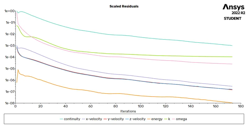
Processor Temperature:

Heat Transfer Coefficient:

Temperature Contour:

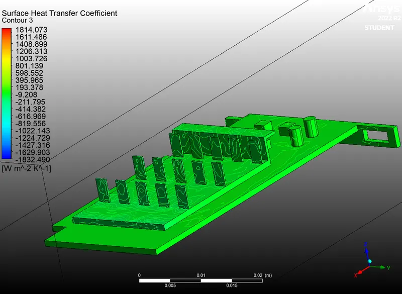
Heat transfer coefficient:

Velocity Vector:

Results:

	Baseline V=1m/s	Refined V=1m/s	Refined – V=3m/s	Refined – V=5m/s
Processor Temperature (K)	376.83	435.77	369.07	350.51
Wall Heat transfer coefficient processor (W/m2K)	-14.0005	-5.4742	-9.8937	-15.0112

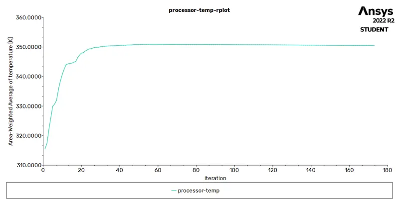
From the above table, we can say that the heat transfer coefficient is rising as the velocity is increasing which is directly related to the greater heat transfer rate. in this model, we want better cooling of graphics card which one can achieved with high inlet velocity (5m/s).

A converged solution for the given sets of input was observed on the basis of repetitive plots in the Residual plot as the difference in the gradients is very small. The processor acted as a source of heat input and thus one of the hotspots for such study.

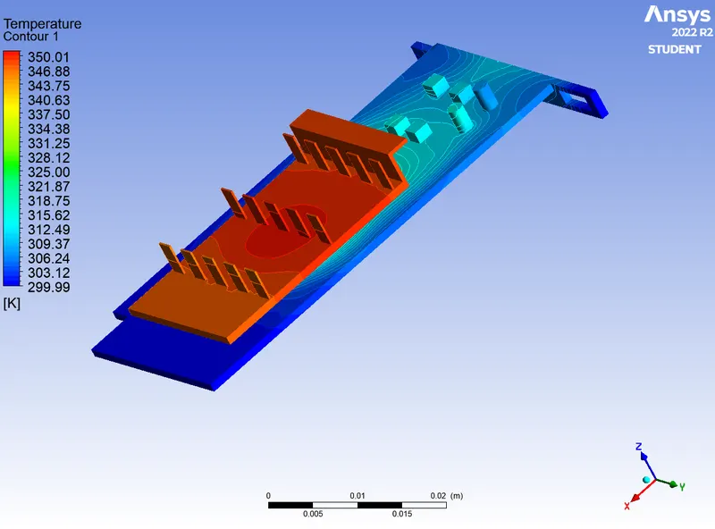
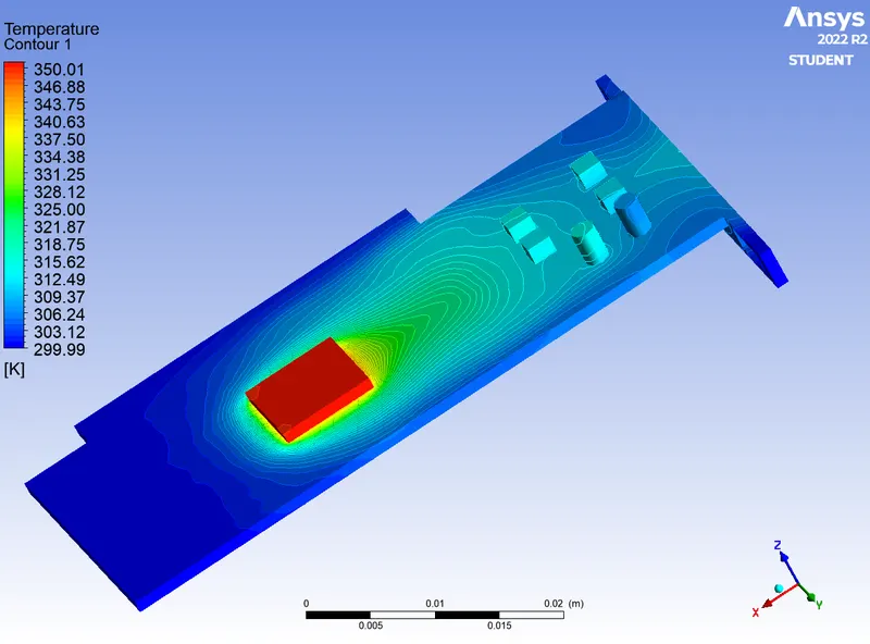
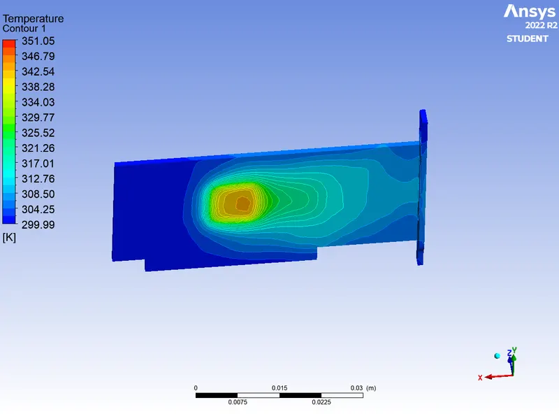
From the temperature distribution, we can see hotspots in the fin and base near the surface that is in contact with the processor. Based on the thermal conductivity of the material this temperature is distributed accordingly amongst the component. We see a few high-temperature zones on fin away from processor depicting their high susceptibility to heat due to their geometry.

Conclusion:

• Higher velocity in a particular region means a higher Reynolds number. That’s why the heat transfer coefficient in that area is highest, which means the maximum amount of heat transfer is taking place from fluid to the solid in that region. This also results in a higher temperature of solid in that location.
• Heat transfer coefficient is a function of properties of the fluid at film temperature, temperature difference, temperature coefficient, buoyance force et, hence, mesh resolution near walls usually has the biggest impact on numerical results.
• For the turbulent models, we have to take care of the assumptions and the boundary conditions you put in the program. The mesh is a very important parameter to get nice results so we have to refine it in the important place of our drawing.
• Some factors should be considered which the most significant is the turbulent boundary layer. If we are using any kind of low Reynolds turbulence model considering enhanced wall treatment (as your K-w SST model), so we need to make sure that we stay in the laminar sub-layer region where velocity profiles are assumed to be laminar and viscous stress dominates the wall shear which means
• Mesh/ grid dependency test is very important to get confidence over results