Deriving 4th order approximation of a 2nd order derivative using Taylor Table method
OBJECTIVE:
The objective of this project is to derive and evaluate a second order derivative of a function by using Taylor’s Tabel method.
The taylor table method is used to simplify the algebraic equation derived using Taylor series and to reduce processing time.
Deriving the 4th Order Approximation of the 2nd order derivative:
- Central difference scheme.
The no of nodes required in this scheme can be solved by using this formula
N=P+Q-1
Where, N is no of nodes
P is the order of approximation
Q is the order of derivative
N=4+2-1=5. So, here we need 5 nodes.
The numerical stencil of central difference scheme:
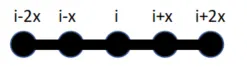
Now the value of `(delta^2f )/( deltax^2)` of the 4th order approximation can be written as
- `(delta^2f )/( deltax^2)=(af(i-2)+bf(i-1)+cf(i)+df(i+1)+ef(i+2)`
By using taylor’s series method we can expand the above equation:
- `af(i-2)=af(i)-2aDeltaxf'(i)+a(2Deltax)^2/(2!)f''(i)-a(2Deltax)^3/(3!)f'''(i)+a(2Deltax)^4/(4! )f'''''(i)`
- `bf(i-1)=bf(i)-bDeltaxf'(i)+b(Deltax^2)/(2!)f''(i)-b(Deltax^3)/(3!)f'''(i)+b(Deltax^4)/(4!)f''''(i)`
- `cf(i)=cf(i)`
- `df(i+1)=df(i)+dDeltaxf'(i)+d(Deltax^2)/(2!)f''(i)+d(Deltax^3)/(3!)f'''(i)+d(Deltax^4)/(4!)f''''(i)`
- `ef(i+2)=ef(i)+2eDeltaxf'(i)+e(2Deltax)^2/(2!)f''(i)+e(2Deltax)^3/(3!)f'''(i)+e(2Deltax)^4/(4! )f'''''(i)`
Since the distance between ¡ to ¡+2 is 2 we are using `2Deltax` and for ¡ to ¡+3 we are using `3Deltax` as well as for ¡+4 . We only need values till of `Deltax^2` so we are assuming the sum of all the values in `Deltax^2` as 1 and for the remaining we are assuming as 0.
Taylor’s table for central differencing:
|
Taylor’s Table |
||||||
|
Assumed functions |
Taylor series expansion |
|||||
|
`f(i)` |
`Deltaxf'(i)` |
`Deltax^2f''(i)` |
`Deltax^3f'''(i)` |
`Deltax^4f''''(i)` |
||
|
Numerical stencil |
`af(i-2)` |
`a` |
`-2a` |
`(4a)/2` |
`-(8a)/6` |
`(16a)/24` |
|
`bf(i-1)` |
`b` |
`-b` |
`b/2` |
`-b/6` |
`b/24` |
|
|
`cf(i)` |
`c` |
`0` |
`0` |
`0` |
`0` |
|
|
`df(i+1)` |
`d` |
`d` |
`d/2` |
`d/6` |
`d/24` |
|
|
`ef(i+2)` |
`e` |
`2e` |
`(4a)/2` |
`(8e)/6` |
`(16e)/24` |
|
|
Sum of coefficients |
`0` |
`0` |
`1` |
`0` |
`0` |
|
From the tabel:
`a+b+c+d+e=0`
`-2a-b+0c+d+2e=0`
`(4a)/2+b/2+0c+d/2+(4e)/2=1`
`-(8a)/6-b/6+0c+d/6+(8e)/6=0`
`(16a)/24+b/24+0c+d/24+(16e)/24=0`
Writing the coefficients in the form of matrix to solve for a,b,c,d and e.
`A=[[1,1,1,1,1], [-2,-1,0,1,2],[2,1/2,0,1/2,2],[-4/3,-1/6,0,1/6,4/3],[2/3,1/24,0,1/24,2/3]]`
`E=[[0],[0],[1],[0],[0]]`
B=inv(A)*E;
`B=[[-0.0833],[1.3333],[-2.5000],[1.3333],[-0.8333]]`
- Skewed right sided difference scheme:
The no of nodes required in this scheme can be solved by using this formula
N=P+Q.
Where, N is no of nodes
P is the order of approximation
Q is the order of derivative
N=4+2=6. So, here we need 6 nodes.
The numerical stencil of skewed right or skewed forward sided difference scheme.
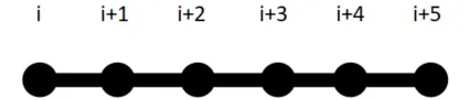
Now the value of `(deltax^2f)/(deltax^2)`of the 4th order approximation can be written as
- `(delta^2f )/( deltax^2)=(af(i)+bf(i+1)+cf(i+2)+df(i+3)+ef(i+4)+gf(i+5)`
By using taylor's series method we can expand the above equation.
- `af(i)=af(i)`
- `bf(i+1)=bf(i)+bDeltaxf'(i)+b(Deltax^2)/(2!)f''(i)+b(Deltax^3)/(3!)f'''(i)+b(Deltax^4)/(4!)f''''(i)+b(Deltax^5)/(5!)f'''''(i)`
- `cf(i+2)=cf(i)+2cDeltaxf'(i)+c(2Deltax)^2/(2!)f''(i)+c(2Deltax)^3/(3!)f'''(i)+c(2Deltax)^4/(4! )f'''''(i)+c(2Deltax)^5/(5!)f'''''(i)`
- `df(i+3)=df(i)+3dDeltaxf'(i)+d(3Deltax^2)/(2!)f''(i)+d(3Deltax^3)/(3!)f'''(i)+d(3Deltax^4)/(4!)f''''(i)+d(3Deltax^5)/(5!)f'''''(i)`
- `ef(i+4)=ef(i)+4eDeltaxf'(i)+e(4Deltax)^2/(2!)f''(i)+e(4Deltax)^3/(3!)f'''(i)+e(4Deltax)^4/(4! )f'''''(i)+e(4Deltax^5)/(5!)f'''''(i)`
- `gf(i+5)=gf(i)+5gDeltaxf'(i)+g(5Deltax)^2/(2!)f''(i)+g(5Deltax)^3/(3!)f'''(i)+g(5Deltax)^4/(4! )f'''''(i)+g(5Deltax^5)/(5!)f'''''(i)`
Since the distance between ¡ to ¡+2 is 2 we are using `2Deltax` and for ¡ to ¡+3 we are using `3Deltax` as well as for ¡+4 and i-5. We only need values till of `Deltax^2` so we are assuming the sum of all the values in `Deltax^2` as 1 and for the remaining we are assuming as 0.
Taylor’s Tabel for right sided difference:
|
Taylor’s Table |
|||||||
|
Assumed functions |
Taylor series expansion |
||||||
|
`f(i)` |
`Deltaxf'(i)` |
`Deltax^2f''(i)` |
`Deltax^3f'''(i)` |
`Deltax^4f''''(i)` |
`Deltax^5f'''''(i)` |
||
|
Numerical stencil |
`af(i)` |
`a` |
`0` |
`0` |
`0` |
`0` |
`0` |
|
`bf(i+1)` |
`b` |
`b` |
`b/2` |
`b/6` |
`b/24` |
`b/120` |
|
|
`cf(i+2)` |
`c` |
`2c` |
`4c/2` |
`8c/6` |
`16c/24` |
`32c/120` |
|
|
`df(i+3)` |
`d` |
`3d` |
`9d/2` |
`27d/6` |
`81d/24` |
`243d/120` |
|
|
`ef(i+4)` |
`e` |
`4e` |
`16e/2` |
`(64e)/6` |
`256e/24` |
`1024d/120` |
|
|
`gf(i+5)` |
`g` |
`5g` |
`25g/2` |
`125g/6` |
`625g/24` |
`3125g/120` | |
|
Sum of coefficients |
`0` |
`0` |
`1` |
`0` |
`0` |
`0` |
|
From the tabel,writing the coefficients in the form of matrix to solve for a,b,c,d and e:
`J=[[1,1,1,1,1,1],[0,-1,-2,-3,-4,-5],[0,1/2,4/2,9/2,16/2,25/2],[0,-1/6,-8/6,-27/6,-64/6,-125/6],[0,1/24,16/24,81/24,256/24,625/24],[0,-1/120,-32/120,-243/120,-1024/120,-3125/120]]`
`P=[[0],[0],[1],[0],[0],[0]]`
R = inv(J) * P:
`R=[[3.75000],[-12.8333],[17.8333],[-13.0000],[5.0833],[-0.8333]]`
- Skewed Left sided difference scheme.
The no of nodes required in this scheme can be solved by using this formula
N=P+Q.
Where, N is no of nodes
P is the order of approximation
Q is the order of derivative
N=4+2=6. So, here we need 6 nodes.
The numerical stencil of skewed left or skewed backwsrd sided difference scheme.
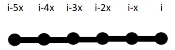
Now the value of `(deltax^2f)/(deltax^2)`of the 4th order approximation can be written as
- `(delta^2f )/( deltax^2)=(af(i)+bf(i-1)+cf(i-2)+df(i-3)+ef(i-4)+gf(i-5)`
By using taylor's series method we can expand the above equation.
- `af(i)=af(i)`
- `bf(i-1)=bf(i)-bDeltaxf'(i)+b(Deltax^2)/(2!)f''(i)-b(Deltax^3)/(3!)f'''(i)+b(Deltax^4)/(4!)f''''(i)-b(Deltax^5)/(5!)f'''''(i)`
- `cf(i-2)=cf(i)-2cDeltaxf'(i)+c(2Deltax)^2/(2!)f''(i)-c(2Deltax)^3/(3!)f'''(i)+c(2Deltax)^4/(4! )f'''''(i)-c(2Deltax)^5/(5!)f'''''(i)`
- `df(i-3)=df(i)-3dDeltaxf'(i)+d(3Deltax^2)/(2!)f''(i)-d(3Deltax^3)/(3!)f'''(i)+d(3Deltax^4)/(4!)f''''(i)-d(3Deltax^5)/(5!)f'''''(i)`
- `ef(i-4)=ef(i)-4eDeltaxf'(i)+e(4Deltax)^2/(2!)f''(i)-e(4Deltax)^3/(3!)f'''(i)+e(4Deltax)^4/(4! )f'''''(i)-e(4Deltax^5)/(5!)f'''''(i)`
- `gf(i-5)=gf(i)-5gDeltaxf'(i)+g(5Deltax)^2/(2!)f''(i)-g(5Deltax)^3/(3!)f'''(i)+g(5Deltax)^4/(4! )f'''''(i)-g(5Deltax^5)/(5!)f'''''(i)`
Since the distance between ¡ to ¡-2 is 2 we are using `2Deltax` and for ¡ to ¡-3 we are using `3Deltax` as well as for ¡-4 and i-5 . We only need values till of `Deltax^2` so we are assuming the sum of all the values in `Deltax^2` as 1 and for the remaining we are assuming as 0.
Taylor’s Tabel for Left sided difference:
|
Taylor’s Table |
|||||||
|
Assumed functions |
Taylor series expansion |
||||||
|
`f(i)` |
`Deltaxf'(i)` |
`Deltax^2f''(i)` |
`Deltax^3f'''(i)` |
`Deltax^4f''''(i)` |
`Deltax^5f'''''(i)` |
||
|
Numerical stencil |
`af(i)` |
`a` |
`0` |
`0` |
`0` |
`0` |
`0` |
|
`bf(i-1)` |
`b` |
`-b` |
`b/2` |
`-b/6` |
`b/24` |
`-b/120` |
|
|
`cf(i-2)` |
`c` |
`-2c` |
`4c/2` |
`-8c/6` |
`16c/24` |
`-32c/120` |
|
|
`df(i-3)` |
`d` |
`-3d` |
`9d/2` |
`-27d/6` |
`81d/24` |
`-243d/120` |
|
|
`ef(i-4)` |
`e` |
`-4e` |
`16e/2` |
`-64e/6` |
`256e/24` |
`-1024d/120` |
|
|
`gf(i-5)` |
`g` |
`-5g` |
`25g/2` |
`-125g/6` |
`625g/24` |
`-3125g/120` | |
|
Sum of coefficients |
`0` |
`0` |
`1` |
`0` |
`0` |
`0` |
|
From the tabel,writing the coefficients in the form of matrix to solve for a,b,c,d and e:
`C=[[1,1,1,1,1,1],[0,1,2,3,4,5],[0,1/2,4/2,9/2,16/2,25/2],[0,1/6,8/6,27/6,64/6,125/6],[0,1/24,16/24,81/24,256/24,625/24],[0,1/120,32/120,243/120,1024/120,3125/120]]`
`F=[[0],[0],[1],[0],[0],[0]]`
L=inv(C)*F;
`L=[[3.75000],[-12.8333],[17.8333],[-13.0000],[5.0833],[-0.8333]]`
MATLAB CODES:
Inputs:
Given Analytical function f(x)=exp(x)*cox(x).
`rArr`Analytical derivative f''(x)=-2exp(x)*sin(x);
Taking x as x=pi/3 and the range of dx varies from pi/4000 to pi/40 with 20 grid points in between them.
- Function Program for Central difference:
function Error_central_differencing=fourth_order_central_differencing(x,dx)
analytical_derivative=-2*exp(x)*sin(x);
funx = @(a) exp(x+(a*dx)) * cos(x+(a*dx));
A=[1 1 1 1 1;-2 -1 0 1 2;2 1/2 0 1/2 2;-4/3 -1/6 0 1/6 4/3;2/3 1/24 0 1/24 2/3];
E=[0;0;1;0;0];
B = inv(A) * E;
central_differencing=B(1)*(funx(-2)) +B(2)*(funx(-1)) +B(3)*(funx(0)) +B(4)*(funx(1)) +B(5)*(funx(2));
central_differencing=central_differencing/dx^2;
Error_central_differencing=abs(central_differencing-analytical_derivative);
end- Function program skewed Right Sidded difference:
function error_right_sided_skew_differencing=fourth_order_right_sided_skew(x,dx)
analytical_derivative = -2*exp(x)*sin(x);
funx = @(a) exp(x+(a*dx)) * cos(x+(a*dx));
J=[1 1 1 1 1 1;0 -1 -2 -3 -4 -5;0 1/2 4/2 9/2 16/2 25/2;0 -1/6 -8/6 -27/6 -64/6 -125/6;0 1/24 16/24 81/24 256/24 625/24;0 -1/120 -32/120 -243/120 -1024/120 -3125/120];
P=[0;0;1;0;0;0];
R = inv(J) * P;
right_sided_skew=R(1)*funx(0) +R(2)*funx(1)+R(3)*funx(2)+R(4)*funx(3)+R(5)*funx(4)+R(6)*funx(5);
right_sided_skew = right_sided_skew/(dx^2);
error_right_sided_skew_differencing=abs(right_sided_skew-analytical_derivative);
end- Function program skewed Left sidded difference:
function error_left_sided_skew_differencing=fourth_order_left_sided_skew(x,dx)
analytical_derivative=-2*exp(x)*sin(x);
funx = @(a) exp(x+(a*dx)) * cos(x+(a*dx));
C=[1 1 1 1 1 1;0 1 2 3 4 5;0 1/2 4/2 9/2 16/2 25/2;0 1/6 8/6 27/6 64/6 125/6;0 1/24 16/24 81/24 256/24 625/24;0 1/120 32/120 243/120 1024/120 3125/120];
F=[0;0;1;0;0;0];
L = inv(C) * F;
left_sided_skew=L(1)*funx(0) +L(2)*funx(-1)+L(3)*funx(-2)+L(4)*funx(-3)+L(5)*funx(-4)+L(6)*funx(-5) ;
left_sided_skew = left_sided_skew/(dx^2);
error_left_sided_skew_differencing=abs(left_sided_skew-analytical_derivative);
end- Main Code:
clear all
close all
clc
x=pi/3;
dx=linspace(pi/4000,pi/40,20);

for i=1:length(dx)
    central_differencing(i)=fourth_order_central_differencing(x,dx(i));
    right_sided_skew(i)=fourth_order_right_sided_skew(x,dx(i));
    left_sided_skew(i)=fourth_order_left_sided_skew(x,dx(i));
end
figure(1)
loglog(dx,central_differencing,'r');
hold on
loglog(dx,right_sided_skew,'k')
hold on
loglog(dx,left_sided_skew,'g')
xlabel('dx')
ylabel('abs error')
legend
legend('central diff','right diff','left diff');
OUTPUT:
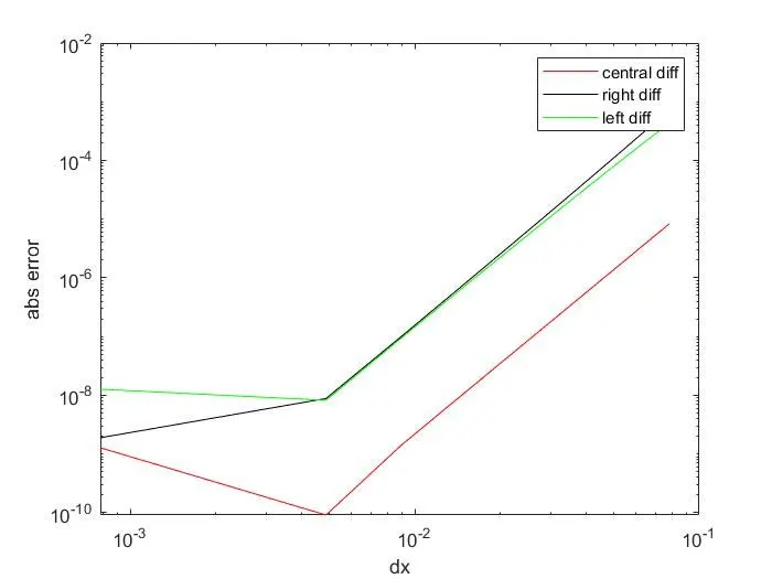
CONCLUSION:
The graph shows that the central differencing scheme is more accurate when compared to other schemes. Therefore the central difference scheme is better than the other schemes.Central difference scheme is more stable than other scheme is because it uses information from both side from point of its consideration. Other schemes has more error and gives less accurate values, because it only uses information only from points of its interest.
Q.Why a skewed scheme is useful?What can a skewed scheme do that a central differencing scheme cannot?
- A skewed scheme can be used on boundary conditions as it takes information from only one direction.
- The CDS cannot be used in boundary conditions because it requires information from both side, so at this condition a skewed scheme is usefull.