Solving the steady and unsteady 2D heat conduction problem

OBJECTIVE:

The objective of this project is to write a MATLAB code to solve 2D heat conduction for steady and unsteady states.

For steady state we are going to solve with three iteratives method.

1. Jacobi Method.
2. Gauss Siedal Method.
3. Successive Over Relaxation Method(SOR).

For unsteady states we are going to use Implicit and Explicit Methods.

SOLUTION:

For steady state 2D Heat conduction equation:

The general 2D temperature equation:

`(delta^2T)/(deltax^2)+(delta^2T)/(deltay^2)=0rarr(1)`

Discretizing the eq(1),with respect to x,we get

`(delta^2T)/(deltax^2)=(T(i-1,j)-2T(i,j)+T(i+1,j))/(dx^2)rarr(2)`

with respect to y, weget,

`(delta^2T)/(deltay^2)=(T(i,j-1)-2T(i,j)+T(i,j+1))/(dy^2)rarr(3)`

Adding eq(2)&eq(3),

`rArr(dy^2(T(i-1,j)-2T(i,j)+T(i+1,j))+dx^2(T(i,j-1)-2T(i,j)+T(i,j+1)))/(dx^2dy^2)=0`

Shuffling according to the common terms,

`(2*T(i,j))/(dx^2)+(2*T(i,j))/(dy^2)=(T(i-1,j)+T(i+1,j))/(dx^2)+(T(i,j-1)+T(i,j+1))/(dy^2)`

Assuming `k=2[(1/dx^2)+(1/dy^2)]`

`rArrk*T(i,j)=(T(i-1,j)+T(i+1,j))/(dx^2)+(T(i,j-1)+T(i,j+1))/(dy^2)`

`rArrT(i,j)=1/k*[(T(i-1,j)+T(i+1,j))/(dx^2)+(T(i,j-1)+T(i,j+1))/(dy^2)]rarr(4)`

where,

T(i,j)=Point

T(i-1,j)=Left boundary

T(i+1,j)=Right boundary

T(i,j+1)=Top boundary

T(i,j-1)=Bottom boundary

from eq(4)

For Jacobi Method:

`T(i,j)^(n+1)=1/k*[(T(i-1,j)+T(i+1,j))/(dx^2)+(T(i,j-1)+T(i,j+1))/(dy^2)]^n`

For Gauss Seidel Method:

`T(i,j)^(n+1)=1/k*[(T(i-1,j)^n+T(i+1,j)^(n+1))/(dx^2)+(T(i,j-1)^(n+1)+T(i,j+1)^n)/(dy^2)]`

For Successive over Relaxation Method:

Here we can use either jacobi method or gauss seidal method, we are using gauss seidal method. And also a relaxation factor alpha is being used.

`T(i,j)^(n+1)=T(i,j)^(n)*(1-alpha)*+alpha*((T(i-1,j)^n+T(i+1,j)^(n+1))/(dx^2)+(T(i,j-1)^(n+1)+T(i,j+1)^n)/(dy^2)]`

MATLAB CODE:

clear all
close all
clc
L=1;
nx=25;
ny=25;
x=linspace(0,L,nx);
y=linspace(0,L,ny);
dx=x(2)-x(1);
dy=y(2)-y(1);
error=9e9;
tol=1e-4;
t=ones(nx,ny);
%given temp
t_top=600;
t_bottom=900;
t_left=400;
t_right=800;
%temp feild
t(1,:)=t_top;
t(end,:)=t_bottom;
t(:,1)=t_left;
t(:,end)=t_right;
%boundary temp
t(1,1)=(t_top+t_left)/2;
t(1,end)=(t_top+t_right)/2;
t(end,1)=(t_left+t_bottom)/2;
t(end,end)=(t_right+t_bottom)/2;
k=2*((dx^2+dy^2)/(dx^2*dy^2));
k1=((dy^2)/(2*((dx^2)+(dy^2))));
k2=((dx^2)/(2*((dx^2)+(dy^2))));
[X,Y]=meshgrid(x,y);
told=t;
%RELAXATION FACTOR
alpha=1.1;
%Iterative method selection
 method=input('Iterative solver=');
    %JACOBI METHOD
    if method==1
        tic;
        jacobi=1;
        while(error>tol)
            for i=2:(nx-1)
                for j=2:(ny-1)
                   term1=(told(i-1,j)+told(i+1,j))/(dx^2);
                   term2=(told(i,j+1)+told(i,j-1))/(dy^2);
                   %t(i,j)=(1-alpha)*told(i,j)+alpha*(k1*tearm1+k2*tearm2);
                   t(i,j)=(term1+term2)/k;
                end
            end
            error=max(max(abs(told-t)));
            told=t;
            jacobi=jacobi+1;
        end
        f=toc;
%Plotting   
figure(1)
[M,N]=contourf(X,Y,t);
clabel(M,N)
colormap(jet)
colorbar
title_1=sprintf('No of iteration:%d',jacobi);
title_2=sprintf('Simulation Time:%f',f);
title({'Jacobi Method';title_1;title_2})
xlabel('x')
ylabel('y')
saveas(figure(1),'JACOBI.jpg')
    end
%GAUSS SEIDAL METHOD
    if method==2
        tic;
        gauss=1;
        while(error>tol)
            for i=2:(nx-1)
                for j=2:(ny-1)
                   term1=(t(i-1,j)+told(i+1,j))/(dx^2);
                   term2=(told(i,j+1)+t(i,j-1))/(dy^2);
                   t(i,j)=(term1+term2)/k;
                end
            end
            error=max(max(abs(told-t)));
            told=t;
            gauss=gauss+1;
        end
        f=toc;
%Plotting
figure(2)
[M,N]=contourf(X,Y,t);
clabel(M,N)
colormap(jet)
colorbar
title_1=sprintf('No of iteration:%d',gauss);
title_2=sprintf('Simulation Time:%f',f);
title({'Gauss Method';title_1;title_2})
xlabel('x')
ylabel('y')
saveas(figure(2),'GAUSS.jpg')
    end
%SOR METHOD
    if method==3
        tic;
        sor=1;
        while(error>tol)
            for i=2:(nx-1)
                for j=2:(ny-1)
                    term1=(t(i-1,j)+told(i+1,j))/(dx^2);
                   term2=(told(i,j+1)+t(i,j-1))/(dy^2);
                   t(i,j)=(term1+term2)/k;
                   t(i,j)=((1-alpha)*(told(i,j)))+(alpha*t(i,j));
                end
            end
            error=max(max(abs(told-t)));
            told=t;
            sor=sor+1;
        end
        f=toc;  
%PlOTTING
figure(3)
[M,N]=contourf(X,Y,t);
clabel(M,N)
colormap(jet)
colorbar
title_1=sprintf('No of iteration:%d',sor);
title_2=sprintf('Simulation Time:%f',f);
title({'sor Method';title_1;title_2})
xlabel('x')
ylabel('y')
saveas(figure(3),'SOR.jpg')
    end

Code explanation:

• First assuming the values for x and y.Then the error and tolerence value is determined.
• Then the given temperatures are defined to their respective feilds, the the boundary temperature values are defined.
• Then the 2-D grid coordinates based on the coordinates contained in vectors x and y are copied in a matrix [X,Y] X is a matrix where each row is a copy of x, and Y is a matrix where each column is a copy of y. using meshgrid.
• The relaxation factor for SOR method is defined.
• An a iterative method input is determined for calling the different inputs.
• Then a convergence loop is called within the convergenge loop a while loop is called where error>tol.
• For calculating each value of i and j Two for loops are called because this is 2D problem.
• Then the error is calculated, and old value t is updated.
• Every iteration is simulated as the above mentioned formate.
• Then atlast graphs are plotted.

OUTPUTS:

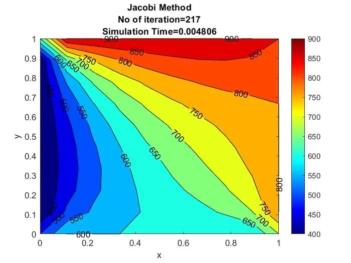
JACOBI METHOD:

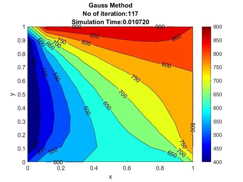
GAUSS SEIDAL METHOD:

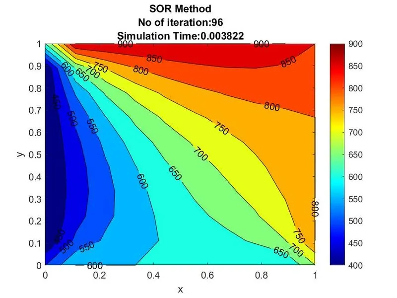
FOR SOR METHOD:

REULTS:

From the outputs we can say that SOR method is the most effcient as it hase low simulation time and number of iterations when compared to other methods. The SOR method has low simulation time and no of iterations because it has a factor called relaxation factor Alpha. The over relaxtion factor is experimented to obtain the efficient solution. In this case after experimenting we are taking the relaxation factor alpha as 1.1 to reach the efficient solution.

TRANSIENT STATE :

For transient state we are going to use two methods,

1. Explicit method.
2. Implicit method.

EXPLICIT METHOD:

The general 2D temperature equation

`alpha*(delta^2T)/(deltax^2)+alpha*(delta^2T)/(deltay^2)=(deltaT)/(deltat)`

Discretizing the above equation:

With respect to x,

`(delta^2T)/(deltax^2)=(T(i-1,j)-2T(i,j)+T(i+1,j))/dx^2`

With respect to y,

`(delta^2T)/(deltay^2)=(T(i,j-1)-2T(i,j)+T(i,j+1))/dy^2`

With respect to time gradient,

`(deltaT)/(deltat)=(T(i,j)^(n+1)-T(i,j)^n)/dt`

Taking the constant terms,

`k1=alpha(dt)/dx^2`

`k2=alpha(dt)/dy^2`

Then the final equation

`T(i,j)^(n+1)=T(i,j)^n+k1(T(i-1,j)-2T(i,j)+T(i+1,j))^n+k2(T(i,j-1)-2T(i,j)+T(i,j+1))^n`

MATLAB CODE:

clear all
close all
clc
L=1;
nx=10;
ny=10;
x=linspace(0,L,nx);
y=linspace(0,L,ny);
dx=x(2)-x(1);
dy=y(2)-y(1);
t=ones(nx,ny);
%given temp
t_top=600;
t_bottom=900;
t_left=400;
t_right=800;
%temp feild
t(1,:)=t_top;
t(end,:)=t_bottom;
t(:,1)=t_left;
t(:,end)=t_right;
%boundary temp
t(1,1)=(t_top+t_left)/2;
t(1,end)=(t_top+t_right)/2;
t(end,1)=(t_left+t_bottom)/2;
t(end,end)=(t_right+t_bottom)/2;
[X,Y]=meshgrid(x,y);
alpha=1.1;
dt=0.001;
total_time=.2;
nt=total_time/dt;
k1=(alpha*dt)/(dx^2);
k2=(alpha*dt)/(dy^2);
cfl=k1+k2;
told=t;
tic;
 iterative_solver=1;
    tic;
    if iterative_solver==1
        iterative_solver=1;
       for p=1:nt
            for i=2:(nx-1)
                for j=2:(ny-1)
                   term1=k1*(told(i-1,j)-2*told(i,j)+told(i+1,j));
                   term2=k2*(told(i,j+1)-2*told(i,j)+told(i,j-1));
                   t(i,j)=told(i,j)+term1+term2;
                   %t(i,j)=(((told(i-1,j)+told(i+1,j))/(dx^2))+((told(i,j+1)+told(i,j-1))/(dy^2)))/k;
                end
            end
            error=max(max(abs(told-t)));
            told=t;
            iterative_solver=iterative_solver+1;
       end
       f=toc;   
figure(1)
[M,N]=contourf(X,Y,t);
clabel(M,N)
colormap(jet)
colorbar
text_1=sprintf('No of iterations=%d ',iterative_solver);
text_2=sprintf(' CFL No=%f',cfl );
text_3=sprintf('Simulation Time taken = %f',f);
title({'Explicit Method';text_1;text_2;text_3})
xlabel('x')
ylabel('y')
saveas(figure(1),'explicit.jpg')
    end

IMPLICIT METHOD:

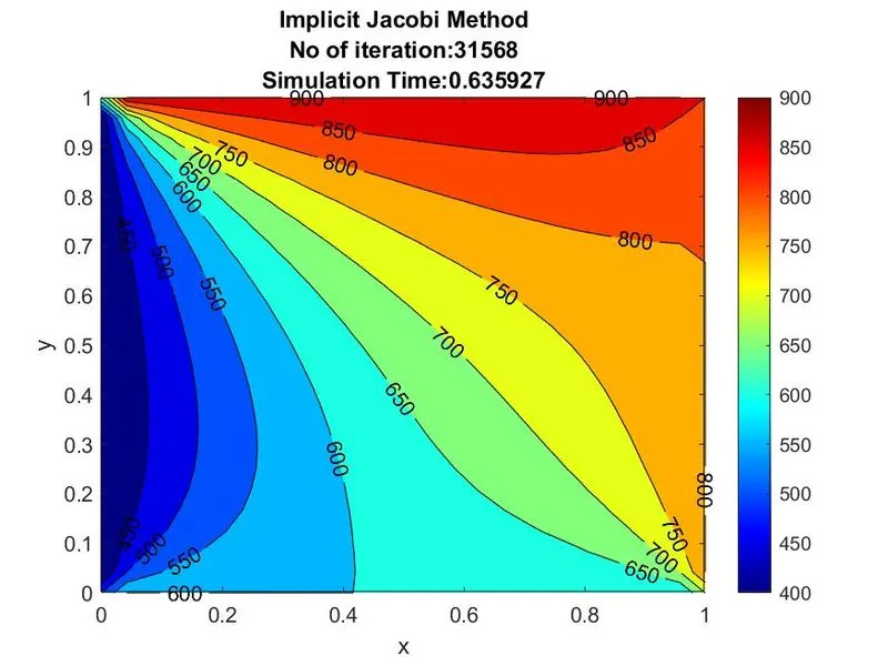
JACOBI METHOD:

`T(i,j)^(n+1)=T(i,j)^n+(k1*(T(i-1,j)+T(i+1,j))^(n)+k2*(T(i,j+1)+T(i,j-1))^n)/(1+2*k1+2*k2)`

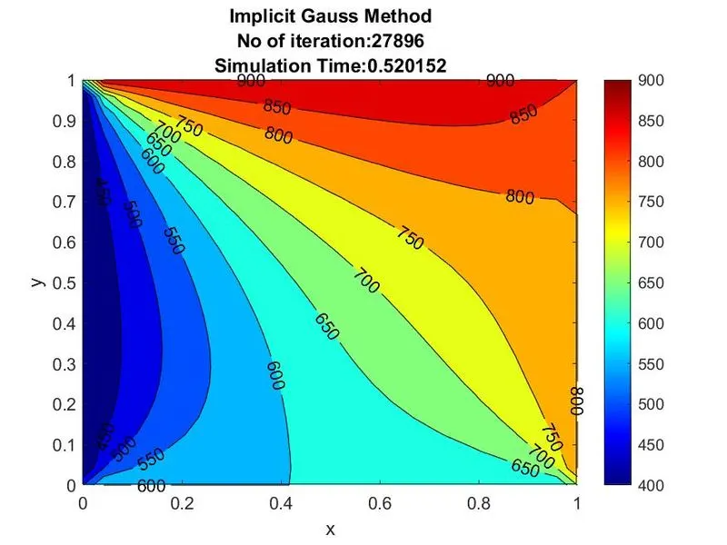
GAUSS SEIDAL METHOD:

`T(i,j)^(n+1)=T(i,j)^n+(k1*(T(i-1,j)^(n+1)+T(i+1,j)^n)+k2*(T(i,j+1)^(n)+T(i,j-1))^(n+1))/(1+2*k1+2*k2)`

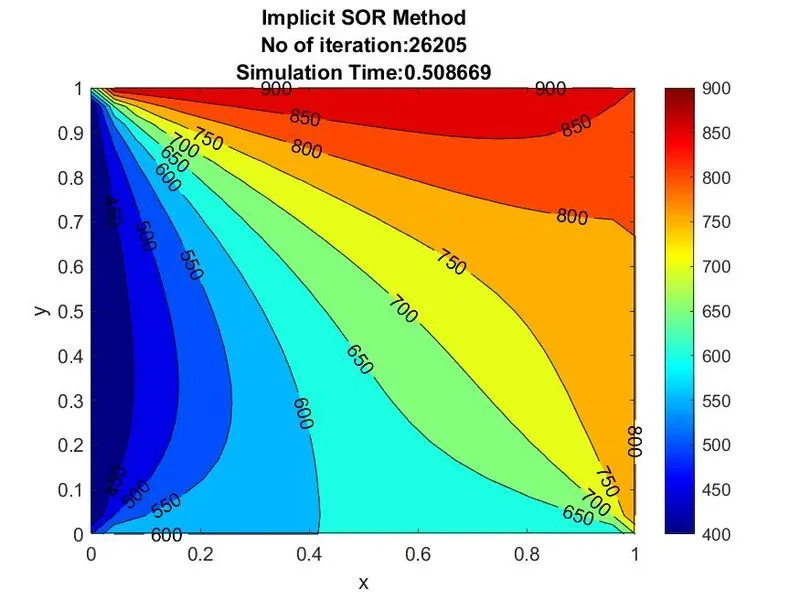
SOR METHOD:

`T(i,j)^(n+1)=T(i,j)^n*(1-omega)+omega*(T(i,j)^n+(k1*(T(i-1,j)^(n+1)+T(i+1,j)^(n))+k2*(T(i,j+1)^(n+1)+T(i,j-1)^n))/(1+2*k1+2*k2))`

clear all
close all
clc
L=1;
nx=25;
ny=25;
x=linspace(0,L,nx);
y=linspace(0,L,ny);
dx=x(2)-x(1);
dy=y(2)-y(1);
error=9e9;
tol=1e-4;
t=ones(nx,ny);
%given temp
t_top=600;
t_bottom=900;
t_left=400;
t_right=800;
%temp feild
t(1,:)=t_top;
t(end,:)=t_bottom;
t(:,1)=t_left;
t(:,end)=t_right;
%boundary temp
t(1,1)=(t_top+t_left)/2;
t(1,end)=(t_top+t_right)/2;
t(end,1)=(t_left+t_bottom)/2;
t(end,end)=(t_right+t_bottom)/2;
dt=0.0001;
[X,Y]=meshgrid(x,y);
told=t;
alpha=0.6;
t_prev_dt=told;
k1=(alpha*dt)/(dx^2);
k2=(alpha*dt)/(dy^2);
CFL_number=k1+k2;
total_time=1;
nt=total_time/dt;
o=1.1;%omega relaxation factor
%iterative method
method=input('Iterative method=');
%Jacobi
if (method==1)
    tic;
    jacobi=1;
    
    for p=1:nt
        
        error=9e9;
        while(error>tol)
            for i=2:(nx-1)
                for j=2:(ny-1)
                    term1=(1+(2*k1)+(2*k2))^-1;
                    term2=k1*term1;
                    term3=k2*term1;
                    h=(told(i-1,j)+told(i+1,j));
                    v=(told(i,j+1)+told(i,j-1));
                    t(i,j)=(t_prev_dt(i,j)*term1)+(term2*h)+(term3*v);
                end                 
            end
            error=max(max(abs(told-t)));
            told=t;
            jacobi=jacobi+1;
        end
        t_prev_dt=t;
    end
    f=toc;
    %plotting
    figure(1)
    [M,N]=contourf(X,Y,t);
    clabel(M,N)
    colormap(jet)
    colorbar
    title_1=sprintf('No of iteration:%d',jacobi);
    title_2=sprintf('Simulation Time:%f',f);
    title({'Implicit Jacobi Method';title_1;title_2})
    xlabel('x')
    ylabel('y')
    saveas(figure(1),'imp jacobi.jpg')
end

%gauss
if (method==2)
    tic
    gauss=1;
    for p=1:nt
        error=9e9;
        while(error>tol)
            for i=2:(nx-1)
                for j=2:(ny-1)
                    term1=(1+(2*k1)+(2*k2))^-1;
                    term2=k1*term1;
                    term3=k2*term1;
                    h=(t(i-1,j)+told(i+1,j));
                    v=(told(i,j+1)+t(i,j-1));
                    t(i,j)=(t_prev_dt(i,j)*term1)+(term2*h)+(term3*v);
                end
            end
            error=max(max(abs(told-t)));
            told=t;
            gauss=gauss+1;
        end
        t_prev_dt=t;
    end
    f=toc;
    %plotting
    figure(2)
    [M,N]=contourf(X,Y,t);
    clabel(M,N)
    colormap(jet)
    colorbar
    title_1=sprintf('No of iteration:%d',gauss);
    title_2=sprintf('Simulation Time:%f',f);
    title({'Implicit Gauss Method';title_1;title_2})
    xlabel('x')
    ylabel('y')
    saveas(figure(2),'imp gauss.jpg')
end

%SOR
if (method==3)
    tic
    sor=1;
    for p=1:nt
        error=9e9;
        while(error>tol)
            for i=2:(nx-1)
                for j=2:(ny-1)
                    term1=(1+(2*k1)+(2*k2))^-1;
                    term2=k1*term1;
                    term3=k2*term1;
                    h=(t(i-1,j)+told(i+1,j));
                    v=(told(i,j+1)+t(i,j-1));
                    t(i,j)=(told(i,j)*(1-o))+(o*((t_prev_dt(i,j)*term1)+(term2*h)+(term3*v)));
                end
            end
            error=max(max(abs(told-t)));
            told=t;
            sor=sor+1;
        end
        t_prev_dt=t;
    end
    f=toc;
    %plotting
    figure(3)
    [M,N]=contourf(X,Y,t);
    clabel(M,N)
    colormap(jet)
    colorbar
    title_1=sprintf('No of iteration:%d',sor);
    title_2=sprintf('Simulation Time:%f',f);
    title({'Implicit SOR Method';title_1;title_2})
    xlabel('x')
    ylabel('y')
    saveas(figure(3),'imp sor.jpg')
end

Code explanation:

• First assuming the values for x and y.Then the error and tolerence value is determined.
• Then the given temperatures are defined to their respective feilds, the the boundary temperature values are defined.
• Then the 2-D grid coordinates based on the coordinates contained in vectors x and y are copied in a matrix [X,Y] X is a matrix where each row is a copy of x, and Y is a matrix where each column is a copy of y. using meshgrid.
• The relaxation factor for SOR method is defined.
• CFL number is also calculated.
• An a iterative method input is determined for calling the different inputs.
• Then a convergence loop is called within the convergenge loop a while loop is called where error>tol.
• For calculating each value of i and j Two for loops are called because this is 2D problem.
• Then the error is calculated, and old value t is updated.
• For implicit method every iteration is simulated as the above mentioned formate.
• Then atlast graphs are plotted.

OUTPUTS:

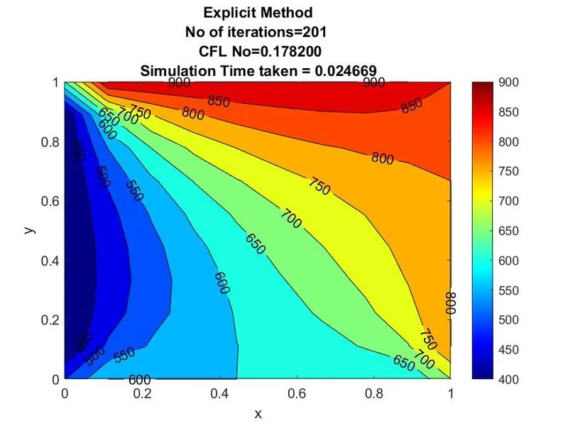
EXPLICIT METHOD:

IMPLICIT METHODS:

JACOBI METHOD:

GAUSS SEIDAL METHOD:

SOR METHOD:

RESULTS:

The results are similar in implicit method as in the steady state method, the sor method gives the most effcient as it has low simulation time and number of iterations when compared to other methods. But the explicit method convergese faster when compared to implicit method