Week 6 - CHT Analysis on a Graphics card

Aim: To Simulate the flow over Graphic card and study Conjugate heat transfer method. Create Heat generation source terms for the processor and to study the temperature around the surrounding components and its effect.

Theory: In order to study air flow around the graphic card, we first need to select the material for the corresponding components

• Flow Fluid = Air
• Fin = Aluminium
• Processor = Silicon
• PCB = FR-4 (composite)

Then we try to define the heat generating source as the processor, for this simulation we take power consumption for the processor to be 10w of which 99.9% is utilized to generate heat. Since the volume for the processor under study is 8 x 8 x 1mm.

Heat generated = Power consumed / Volume of the processor

= 10/(0.008*0.008*0.001)

= 15,62,50,000 w/m^3

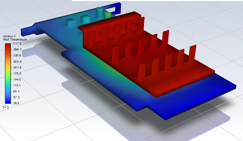
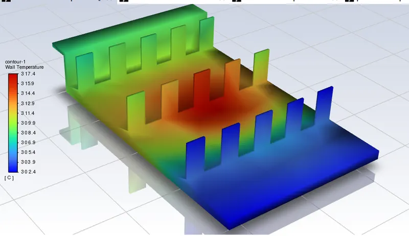
In this simulation we would like to see the temperature distribution around PCB, Processor & Fin. In order to check the air flow over the fin and its capacity to cool the processor. With the current position checking for the hotspots around the PCB.

Baseline Simulation:

• Import the geometry from the saved location and then check for the interference and convert it into share topology.
• Now in the mesh select each component and name them, further Generate the mesh for 0.01m element size.

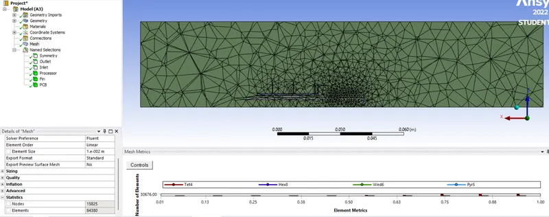
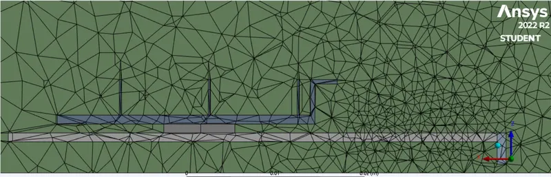
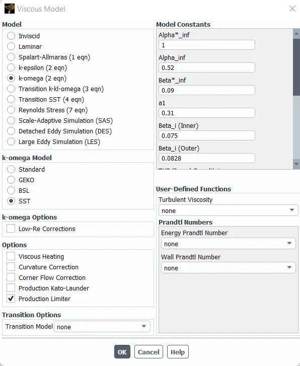
• Select the K-omega turbulence model, then check the energy equation as we are interested in temperature of the components.

Turbulence Model:

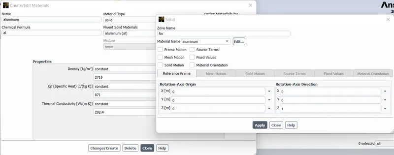
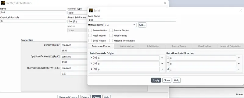
• Create material and assign for the different cell zone.

Working Fluid: Air

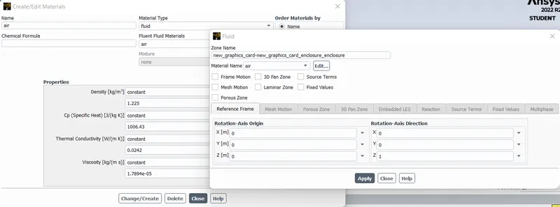
Fin: Aluminium

PCB: FR-4

Processor: Silicon

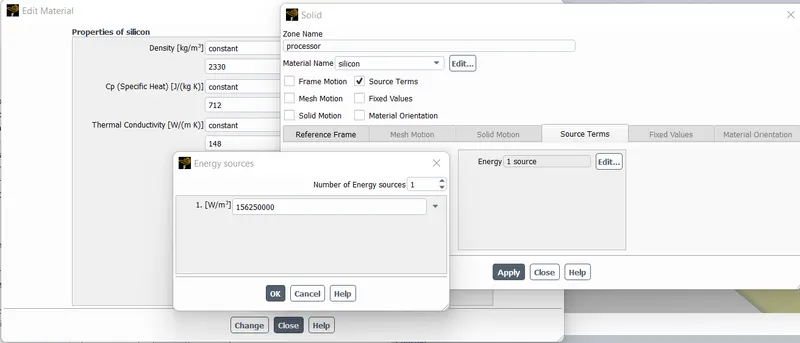
• Assign the processor as heat generation source with the corresponding value.
• Boundary condition, Velocity: 1m/s for inlet & Outlet gauge pressure: 0pa.
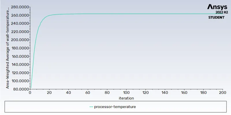
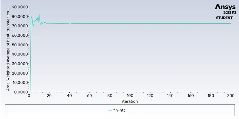
• Generate report for the Area Weighted Average for the processor wall temperature & fin heat transfer coefficient.

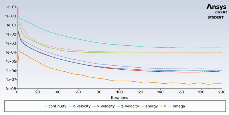
Residual:

Processor Wall Temperature:

Fin Heat Transfer Coefficient:

• Contours for wall temperature of different body.

Temperature Contour:

Fin Temperature:

Processor Temperature:

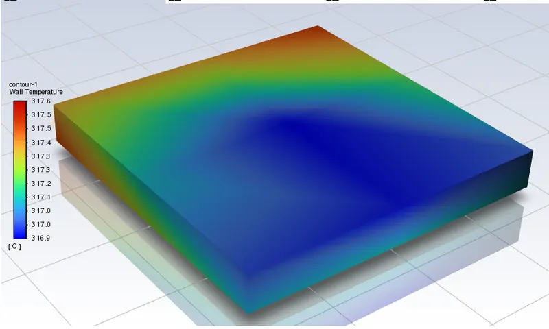
PCB Temperature:

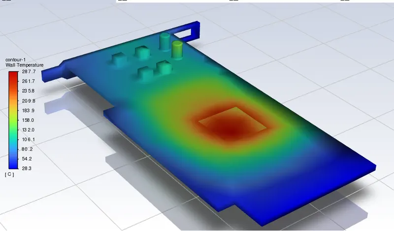
Streamline temperature plot:

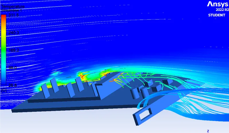
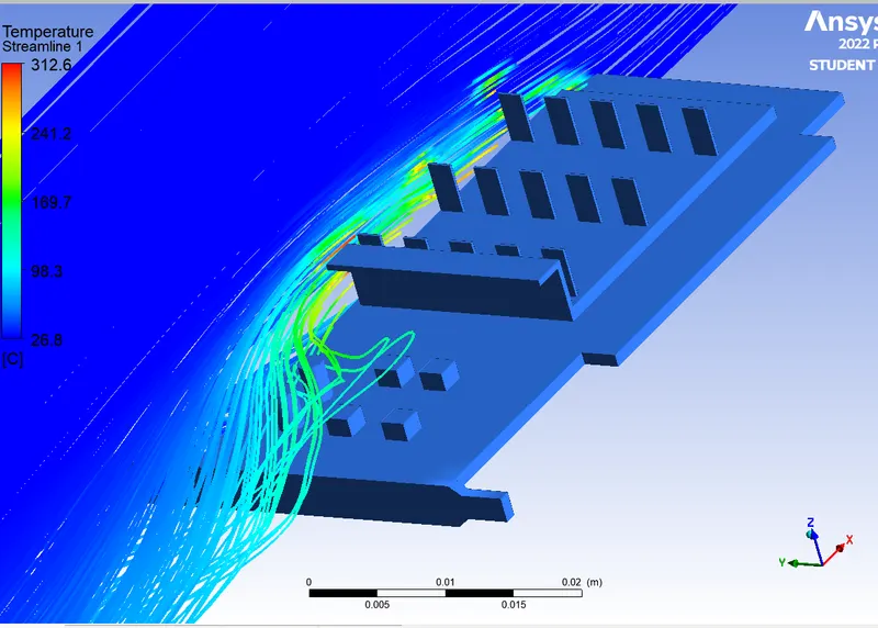
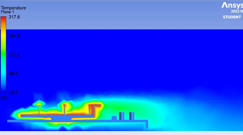
Temperature Contour:

Shell Conduction Method:

• Ansys usually considers zero wall thickness thus considering zero thermal resistance to heat across them. If a thickness is specified for walls then the appropriate thermal reisitance across the wall thickness is imposed wherein the heat transfer takes place normal to the boundary wall.
• Shell conduction is used to model thin sheets without the need to mesh wall thickness in a preprocessor. If shell conduction is applied on the boundary wall the boundary condition that you specify on the original wall is applied to the inner surface and the original wall is treated as coupled wall.
• However internal emissivity is applied at the outer surface. The shell boundaries need boundary condition as well. If the wall with the shell conduction is connected to another wall that has no shell conduction the shell side takes its boundary condition.
• The sides will be adiabatic if they are connected to the face zones having a boundary condition type other than a "wall". If the attached wall has shell conduction the common sides at the junction will be coupled.

Fine Mesh Simulation for 1m/s Inlet Velocity:

• Similar to baseline simulation all condition are same except for the Mesh and following steps.
• As from the baseline results it is seen that temperature gradient are diffused. Hence we need to refine the mesh but within the bounded resource available.
• Assign the element size to be 0.002m and choose Method >> Body sizing for PCB, Processor, Fin with element size to be 0.001m.

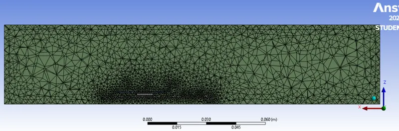
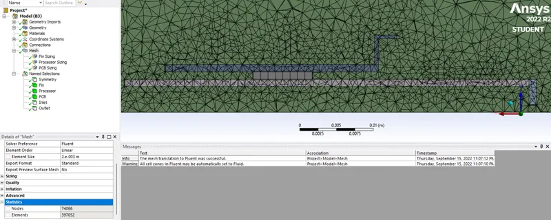
• Define material to different cell zone, then in the boundaries for Processor & Fin select shell conduction.

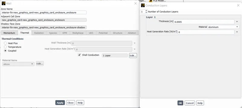
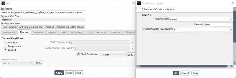
• After assigning the shell conduction the no. of elements increases.
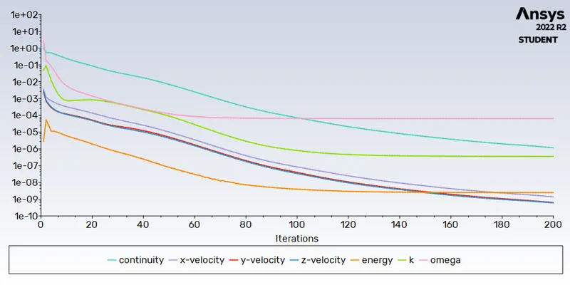
• Similar to baseline simulation generate the results.

Residual:

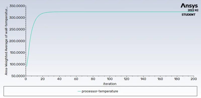
Processor Wall Temperature:

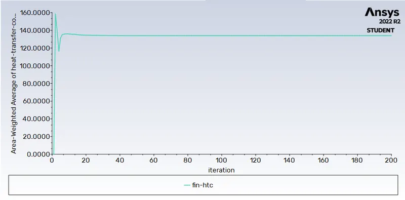
Fin Heat Transfer Coefficient:

Temperature Contour:

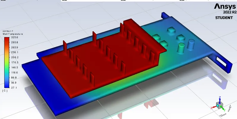
Fin Temperature:

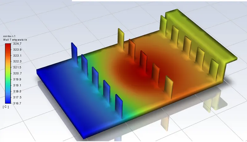
Processor Temperature:

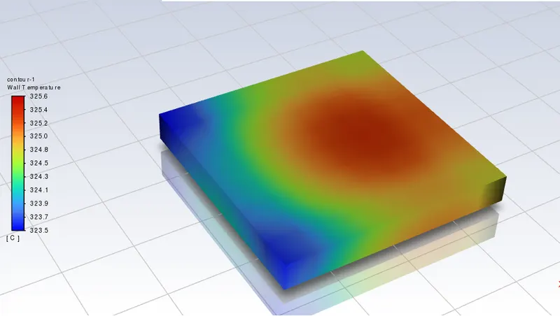
PCB Temperature:

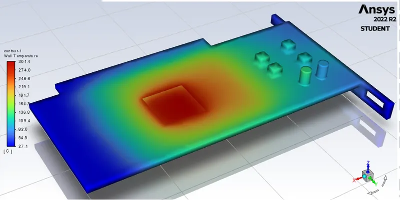
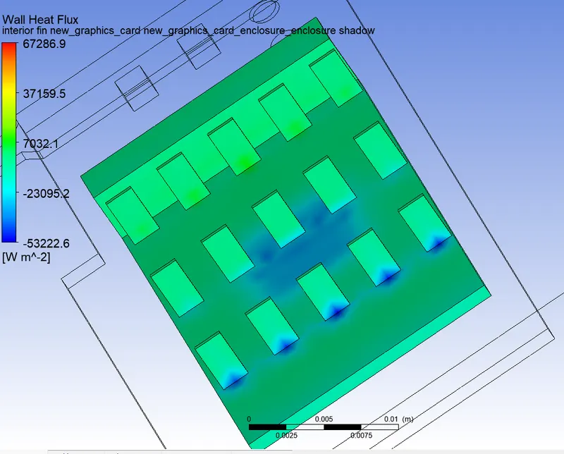
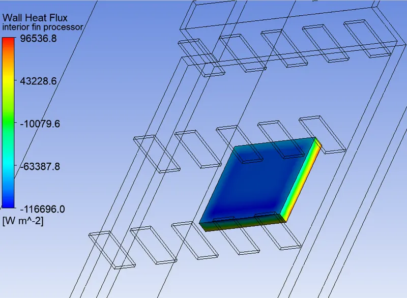
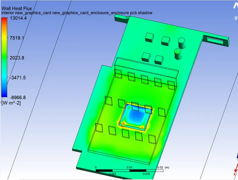
Heatflux:

Streamline temperature plot:

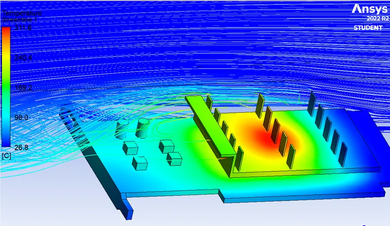
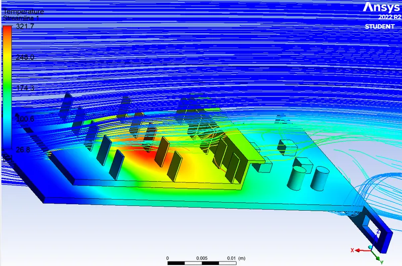
Temperature Contour:

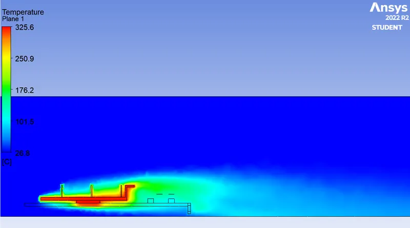
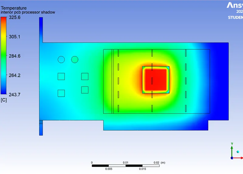
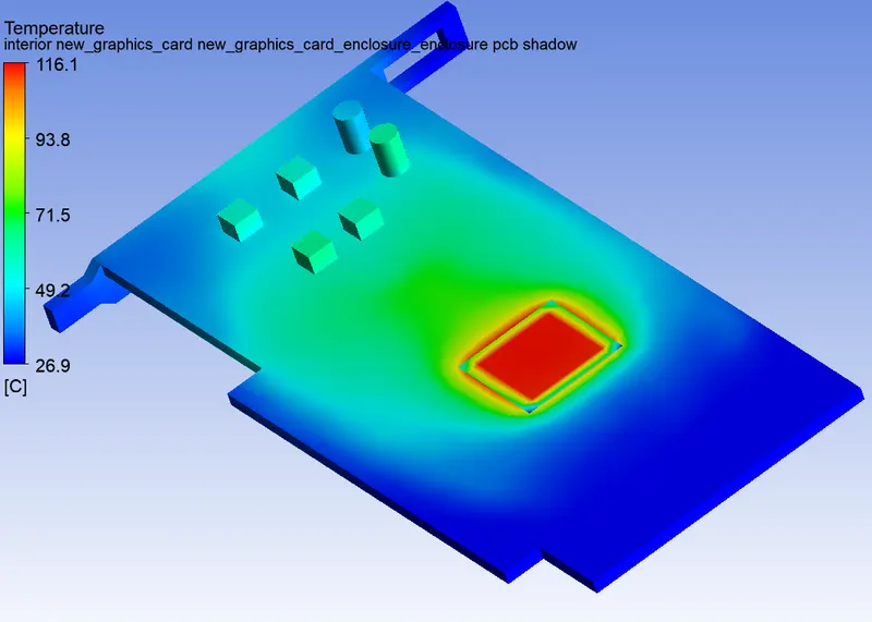
Hotspot Region:

Fine Mesh Simulation for 3m/s Inlet Velocity:

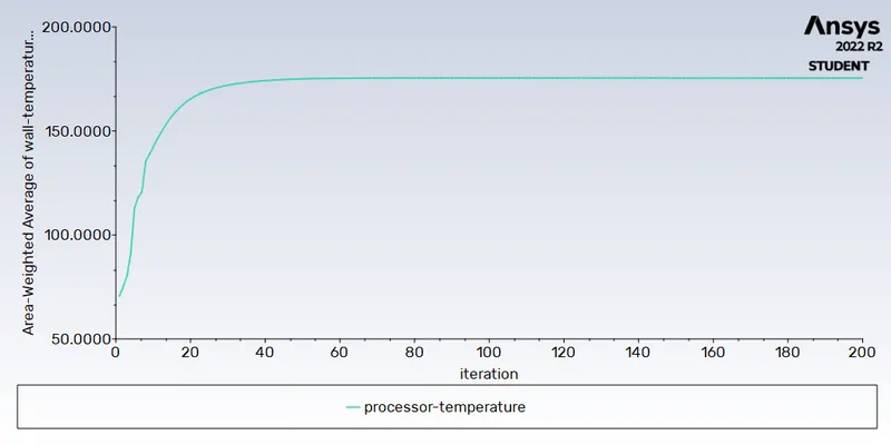
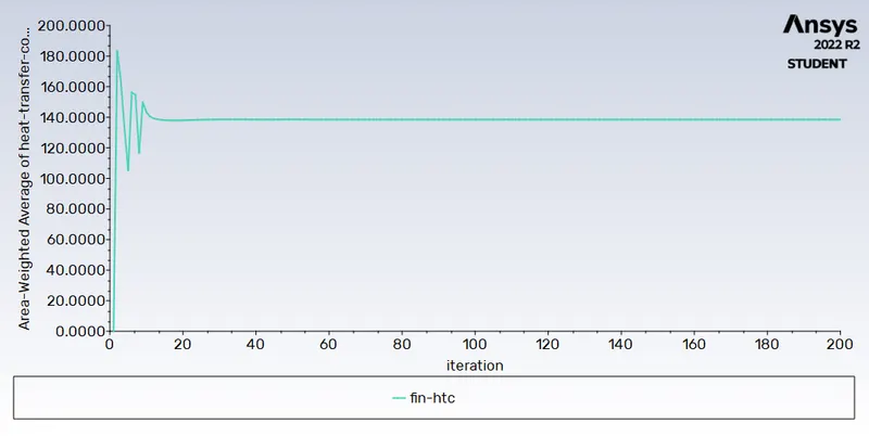
Residual:

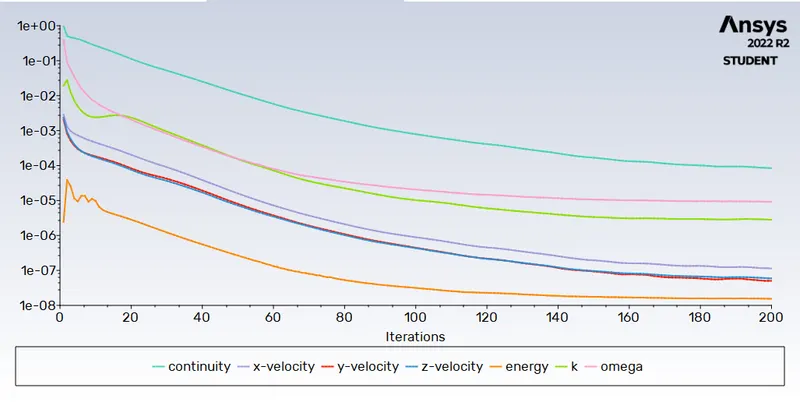
Processor Wall Temperature:

Fin Heat Transfer Coefficient:

Temperature Contour:

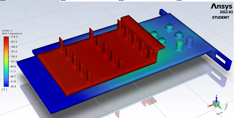
Fin Temperature:

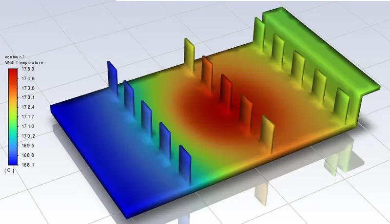
Processor Temperature:

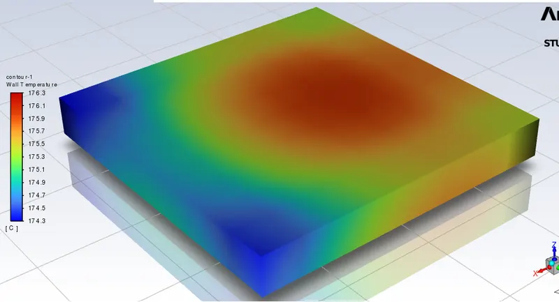
PCB Temperature:

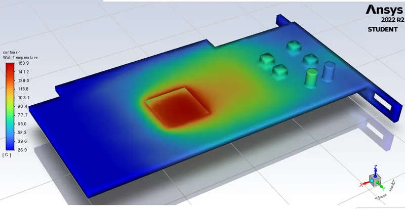
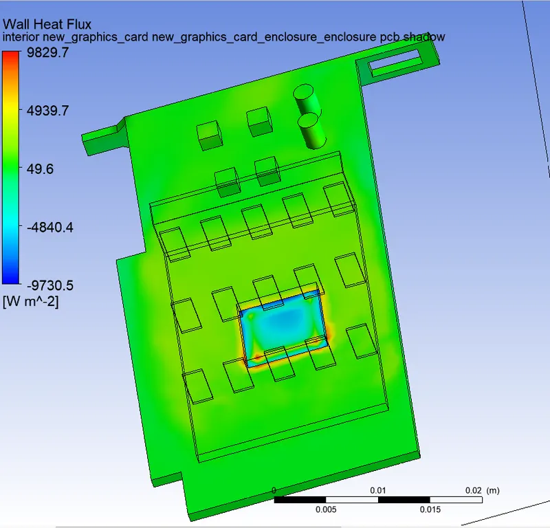
Heatflux:

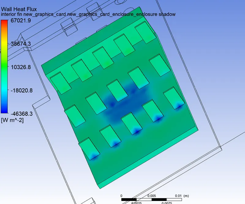
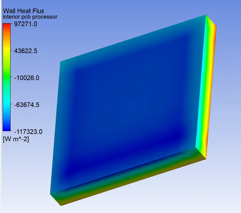
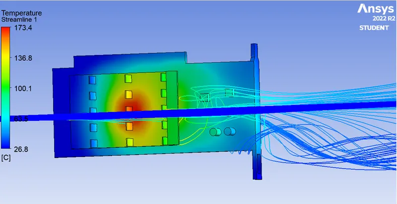
Streamline temperature plot:

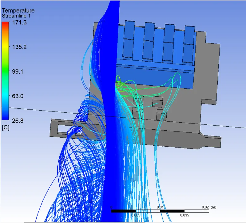
Temperature Contour:

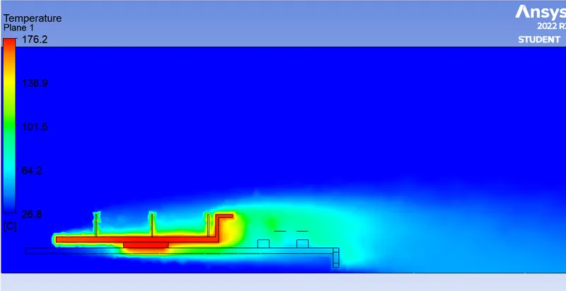
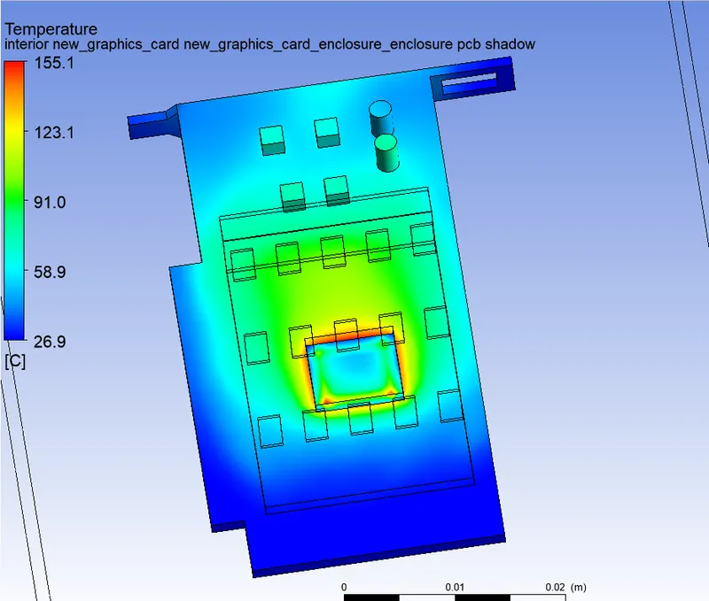
Hotspot

Fine Mesh Simulation for 5m/s Inlet Velocity:

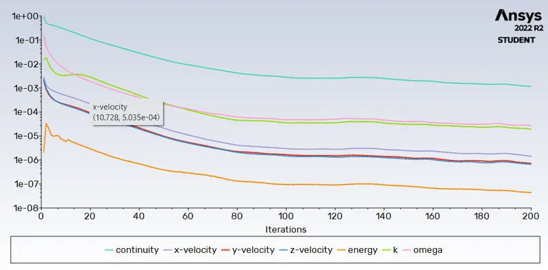
Residual:

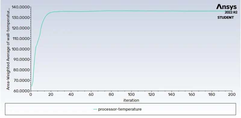
Processor Wall Temperature:

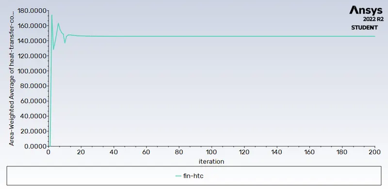
Fin Heat Transfer Coefficient:

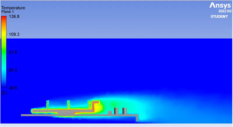
Temperature Contour:

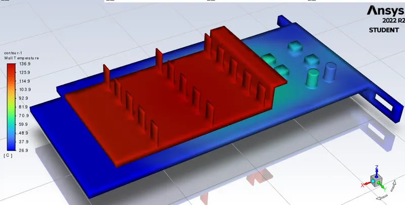
Fin Temperature:

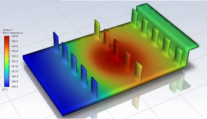
Processor Temperature:

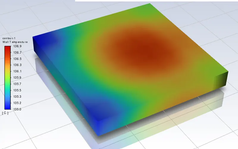
PCB Temperature:

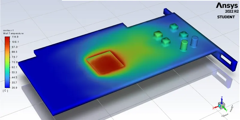
Heatflux:

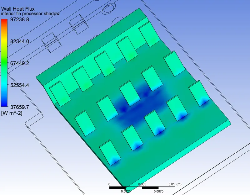
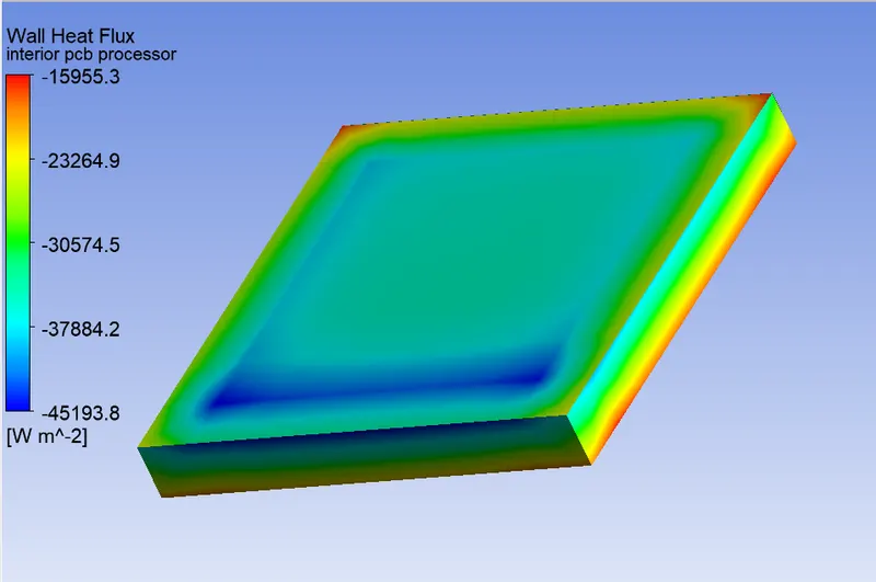
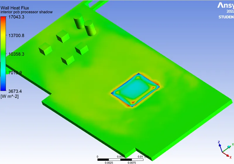
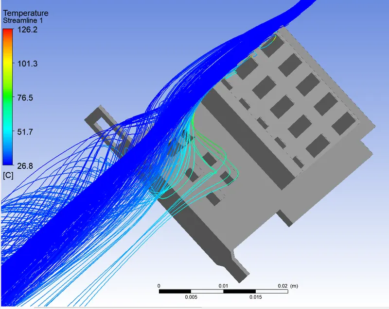
Streamline temperature plot:

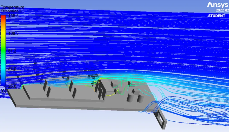
Temperature Contour:

Hotspot

Result:

Velocity	Mesh	Fin HTC	Processor Temperature	Element Size	No. of Element	Iteration
1m/s	Baseline	72.55	263.44*C	0.01m	84,380	200
1m/s	Finer	134.015	324.76*C	0.002m	4,00,820	200
3m/s	Finer	138.498	175.488*C	0.002m	4,00,948	200
5m/s	Finer	145.906	136.084*C	0.002m	4,00,948	200

Conclusion:

• From the above result obtained it is seen that as the Inlet Velocity is increased, Processor temperature starts to decrease. Further as the velcocity is increased fin HTC is also increased.
• From the temperature streamline contour it is found that at the rear of the body air recirculates as a result at this portion heat exchange is reduced. So if in this region any heat generating electronic component is positioned then it will increase its temperature, thus damaging the electronic component.
• From the temperature streamline it is seen that as air flows below the PCB and around the body carries the heat and transport it at the recirculating portion of the Graphic card due to which hotspots arise at various position of the graphic card.