Week 6 - CHT Analysis on a Graphics card

Aim:

To perform comprehensive CHT analysis on a graphics card.

Objectives:

1. Explain the geometry and provide suitable assumptions for the materials and power generation.
2. Generate conformal meshes between the enclosure and the solid body of the graphics card.
3. Simulate the flow problem for 3 inlet velocity conditions (1, 2.5, and 5 m/s) and explain criteria for convergence of the steady state flow.
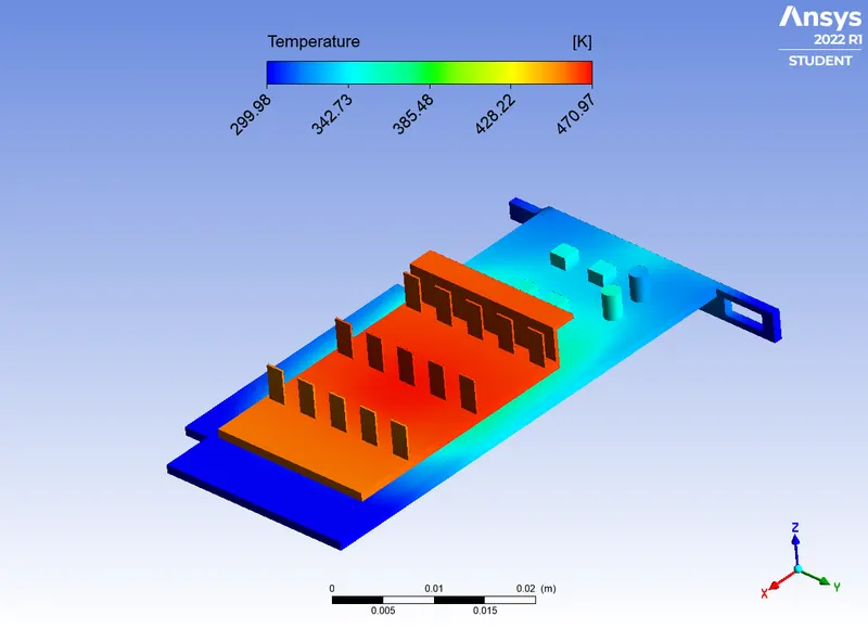
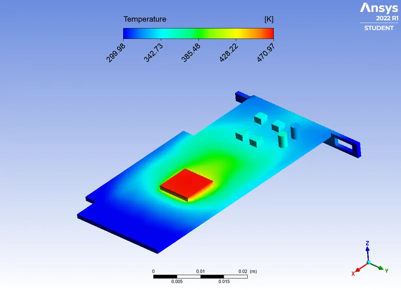
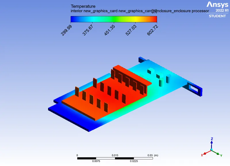
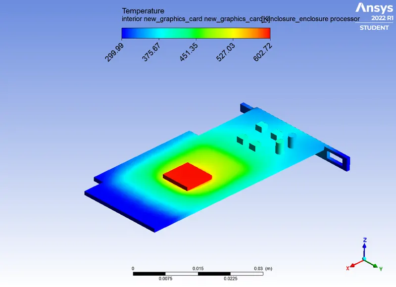
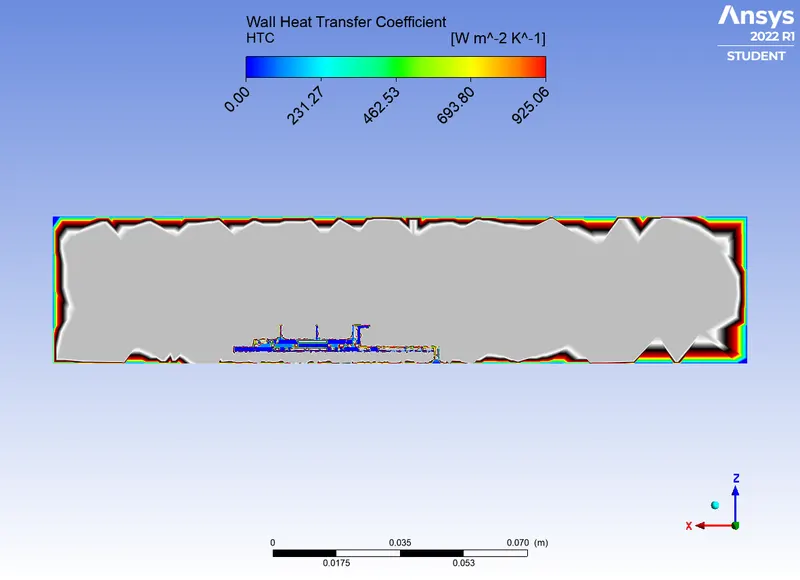
4. Post-process the simulation results to predict the hotspots on the graphic card and wall heat transfer coefficient for the different inlet velocities.

Geometry & Assumptions:

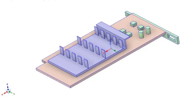
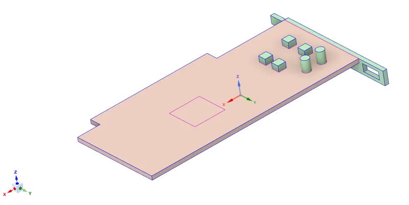
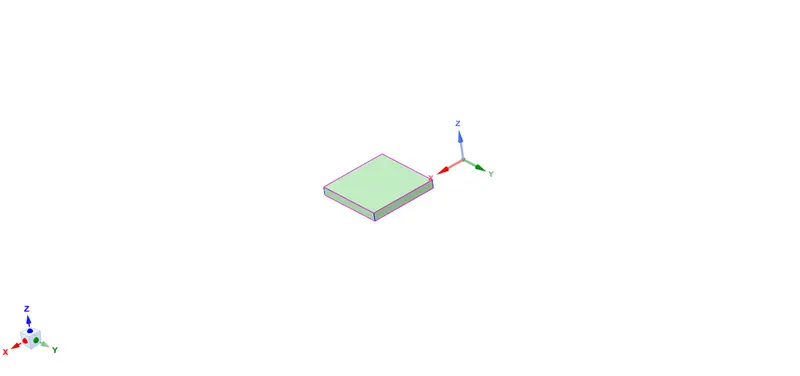
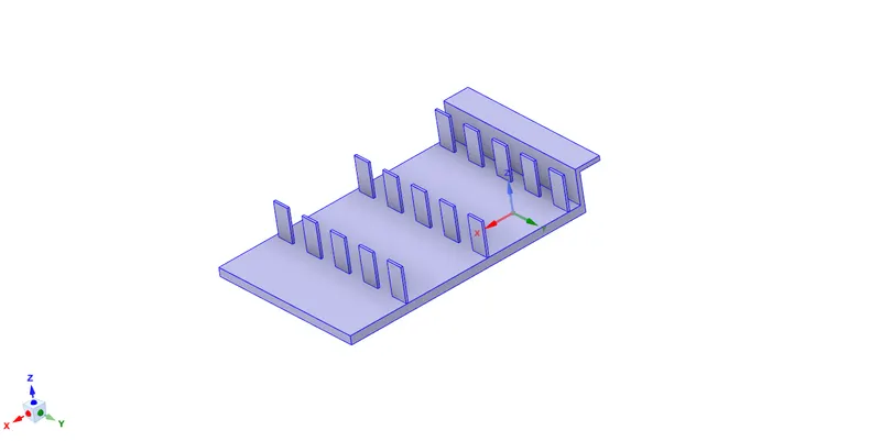
The geometry considered for the current study is a simplified model of the graphics card. The entire card can be classified into three major regions: 1) base of the card, 2) processor and 3) fins. The base of the card includes everything on the card except the processor and cooling component fins. The base is made FR-4 material which is the most commonly used graded synthetic materials for designing PCB. The processor will act as the energy source because of the heat generated due to the supply of the electrical power and is assumed to be made of silicon. The fins provide convective cooling to the processor so that there are no thermal damages on the graphics card. The fins are assumed to made of standard aluminium available in Fluent database.

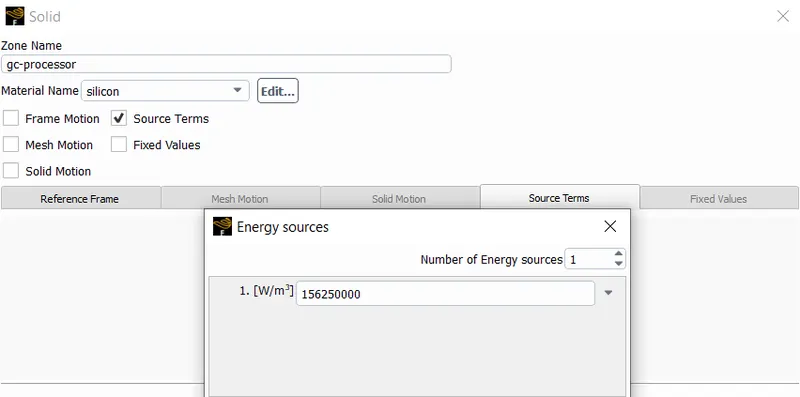
The processor is assumed to be powered with 10 W supply and further its assumed that entire power is converted in thermal energy. Therefore, from simple energy density calculation we can determine the thermal source term.

S=10 W8 mm×8 mm×1 mm=1.5625×108 Wm3S=10 W8 mm×8 mm×1 mm=1.5625×108 Wm3

The working fluid which flows in the enclousre for cooling the card is standard air from the Fluent database. The thermodynamical and physical properties of these materials will be discussed in detail in the Case Setup section.

To solve the Conjugate heat transfer problem, we use the share tool in the Ansys SpaceClaim toolkit, so that we are able to generate conformal mesh. The entire geometry and its components which are discussed above are visualized in the following figures

Graphics Card:

Base of the card:

Processor:

Fins:

Meshing:

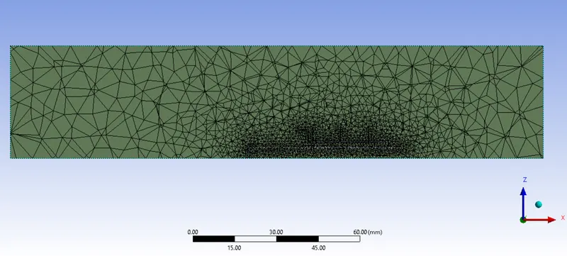
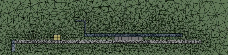
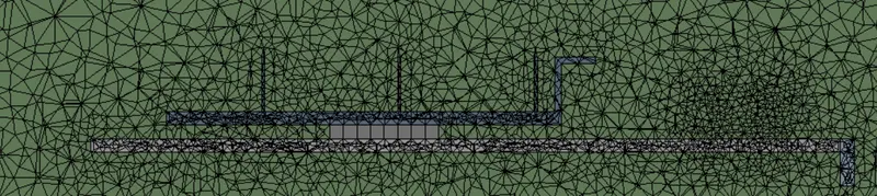
For this study, we considered two types of meshes for understanding the dependence of the grid on the flow parameters. The first mesh is a base mesh generated using default parameters in the Ansys Meshing toolkit. In the baseline mesh, we add face sizing of 5mm as the hybrid initialization of the simulation with default parameters diverged. The second mesh that we use for the simulations has body sizing for each of the components of the graphics card. The enclourse body sizing is of 2.5 mm while the components have a element size of 0.5 mm. Mesh 1 has 174872 elements while the Mesh 2 has 500203 elements.

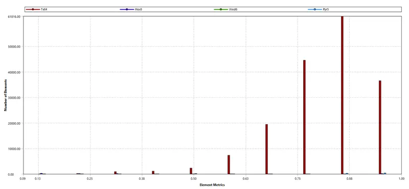
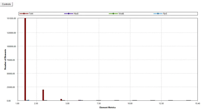
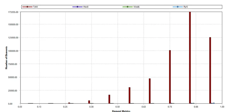
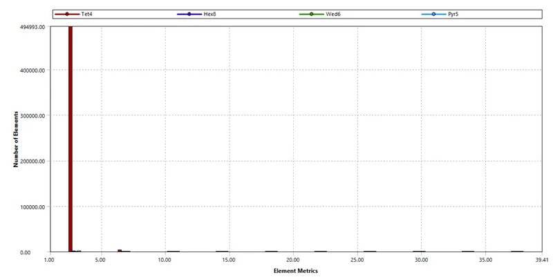
The cut section view of the mesh along with its metrics are shown in the following images.

Mesh 1

• Cutsection view of the geometry

• Closer view on the graphics card

• Mesh Quality

• Aspect ratio

Mesh 2

• Cutsection view of the geometry

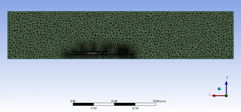
• Closer view of the geometry

• Element Quality

• Aspect Ratio

Case setup:

The case setup is almost identical for all the cases in this study. The settings chosen in the Ansys Fluent GUI are as follows:

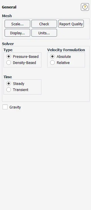
• General
  • Pressure-based, steady state solver is chosen for the study.
  • Volecity formulation is absolute

• Models
  • Since, we are considering heat transfer, the energy equation is used.
  • Turbulence model used is the standard k-ωω SST.
• Materials
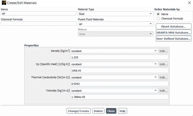
  • The working fluid is the standard air from the Fluent database
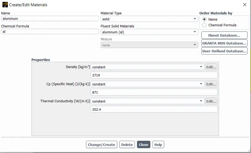
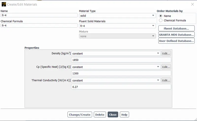
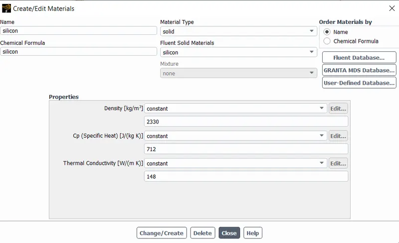
  • As mentioned in the assumptions section, we have chosen FR-4, silicon and aluminium for the PCB board, processor and the cooling fins resepectively.

Air

Alumnium

FR-4 synthetic material

Silicon

• Cell zone conditions
  • The enclosure is filled with the standard air.
  • The base is assigned the FR-4 material and the fins is assigned with aluminium.
  • Along with assigning the silicon to the processor, we provide a source term of 1.5625×108 Wm31.5625×108 Wm3 as derived in the assumptions section.

• Boundary conditions
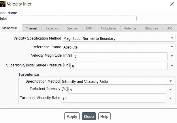
  • Apply 1 or 2.5 or 5 m/s inlet velocity normal to the boundary.
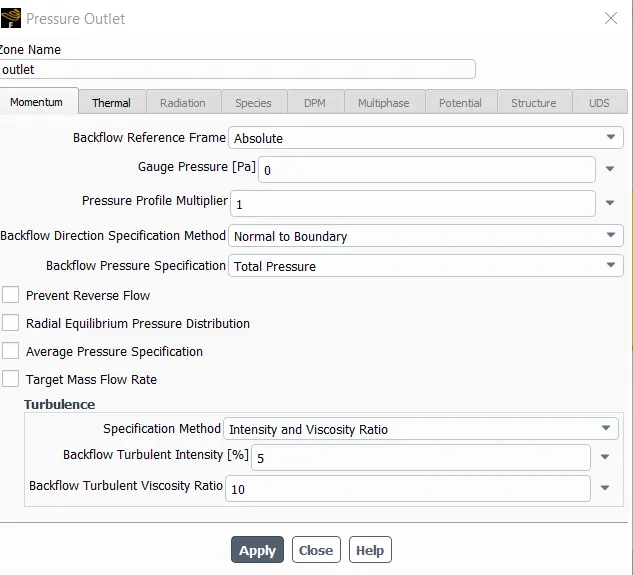
  • Apply 0 gauge pressure for the pressure outlet
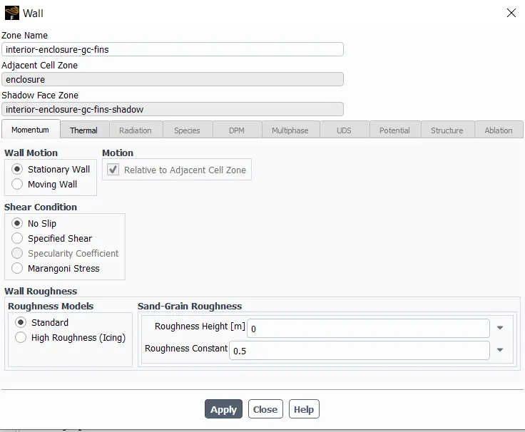
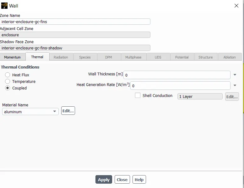
  • Walls are assigned with no-slip boundary conditions and coupled thermal boundary conditions as we are performing CHT simualtions

Inlet

Outlet

Walls: (Ex: Between the fins and the enclosure)

• Report definitions
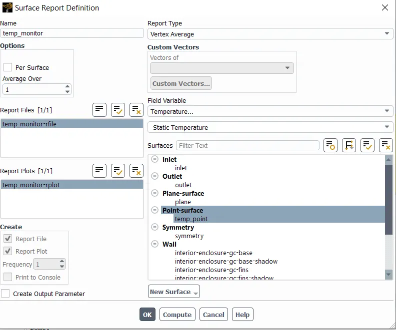
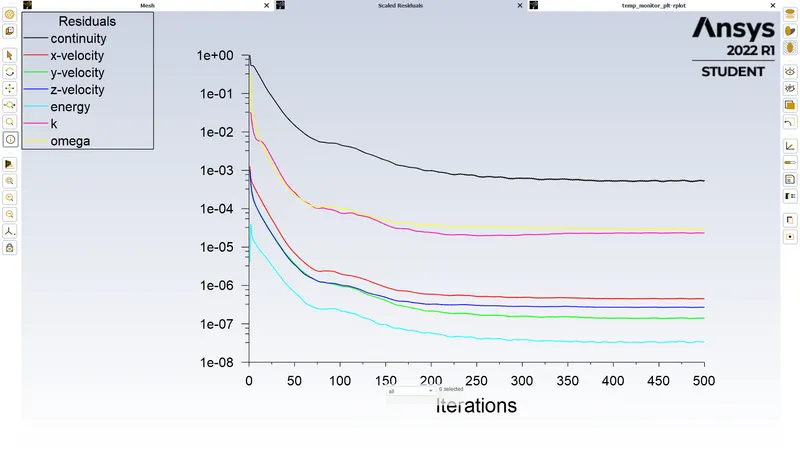
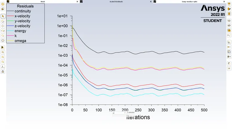
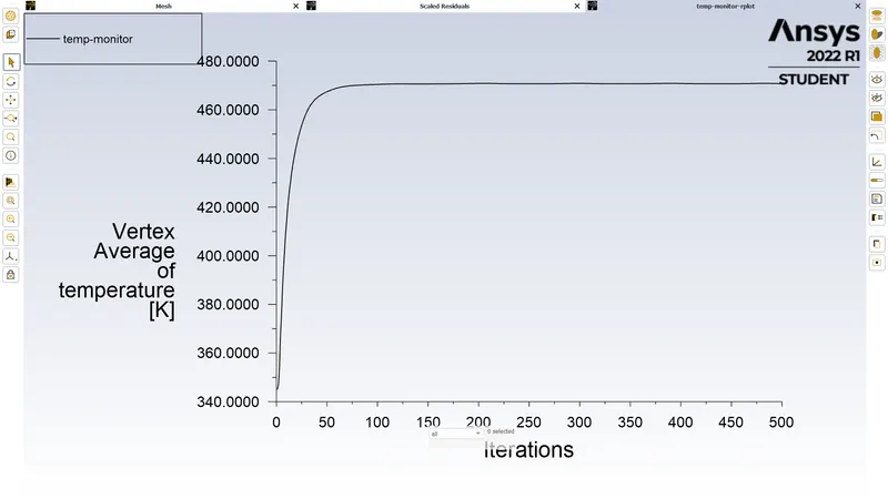
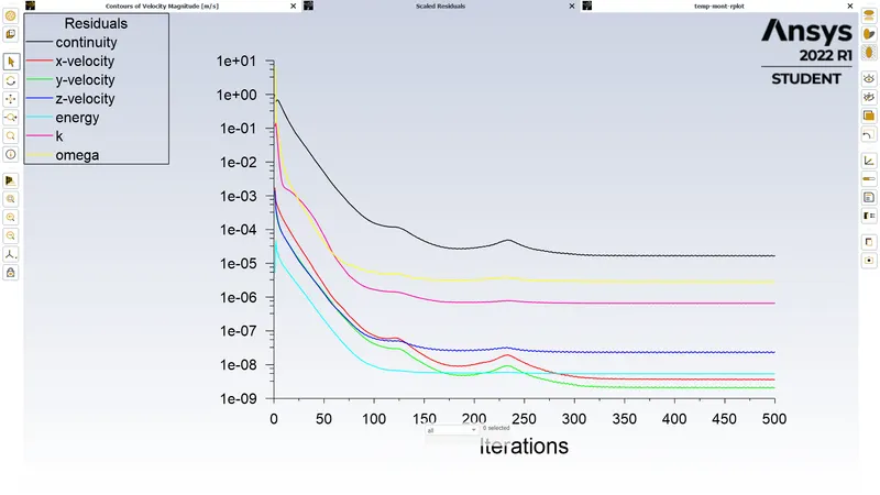
  • It is assumed that the residuals will stagnate and hence cannot be used to identify whether steady state is achieved.
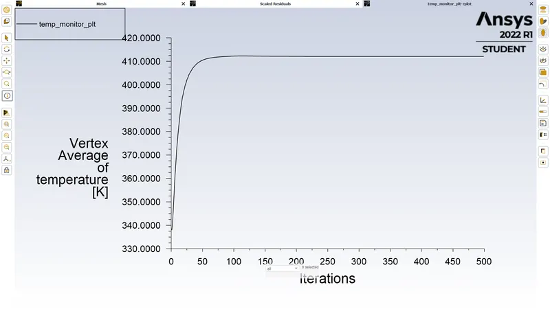
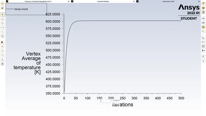
  • A point inside the processor is used to monitor whether the temperature distribution inside has reached the steady state.

• Initialization
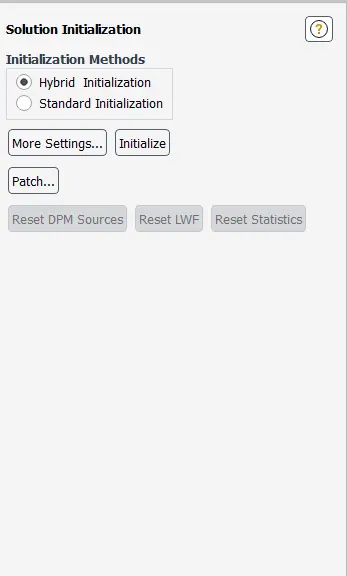
  • The velocity profile in the enclosure is intiialized using 20 iterations of hybrid initialzation.

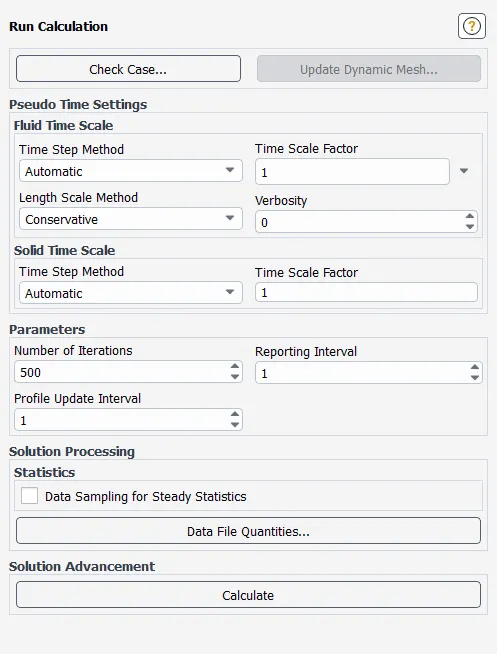
• Run Calculation
  • The simulation is ran for 500 iterations

Grid Dependence:

Before carrying out the comprehensive study on the effects of the inlet velocity on the performance of the cooling systems of the graphics card, we carry out a grid dependance study. This study compares the performance of the two meshes described in the Meshing section and will aid us on deciding which geometry to use for further analysis. The results of the test are summarised in the following table.

Mesh	Number of cells	Temperature of processor (K)	Max velocity (m/s)
Baseline	174872	412.10	6.30
Refined	500203	412.22	6.23

From the above analysis, we can conclude that the baseline mesh is sufficient to resolve the important flow characterisitics and hence we will use the baseline mesh for rest of the study.

Simulation Results:

Inlet velocity of 5m/s

• Residuals vs number of iterations

• Temperature monitor vs number of iterations

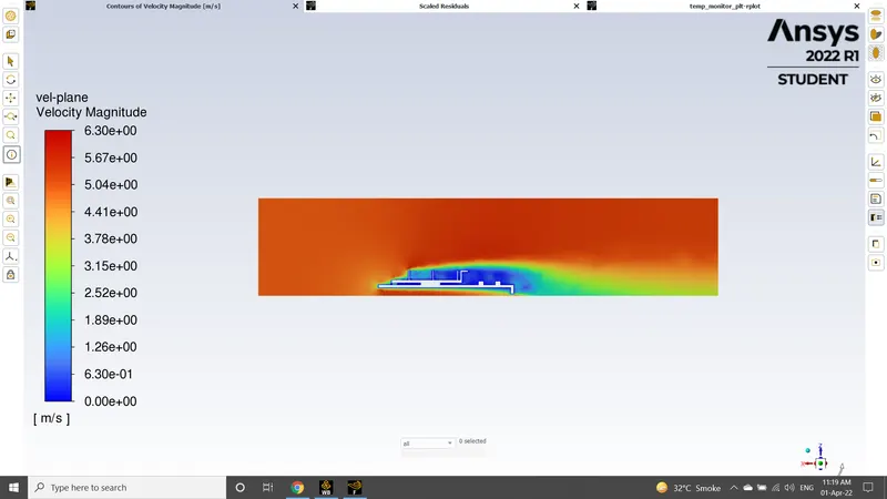
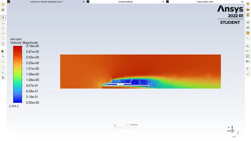
• Steady state velocity contour on plane y = -0.0015 m

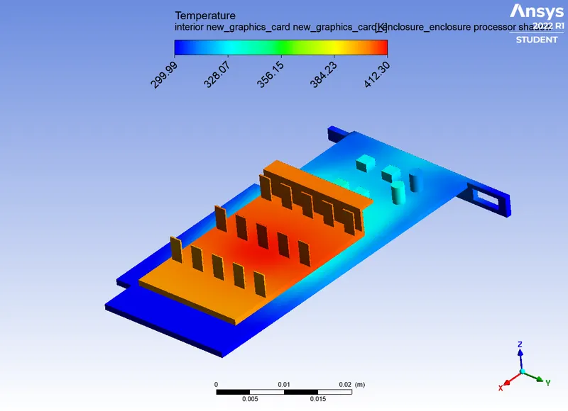
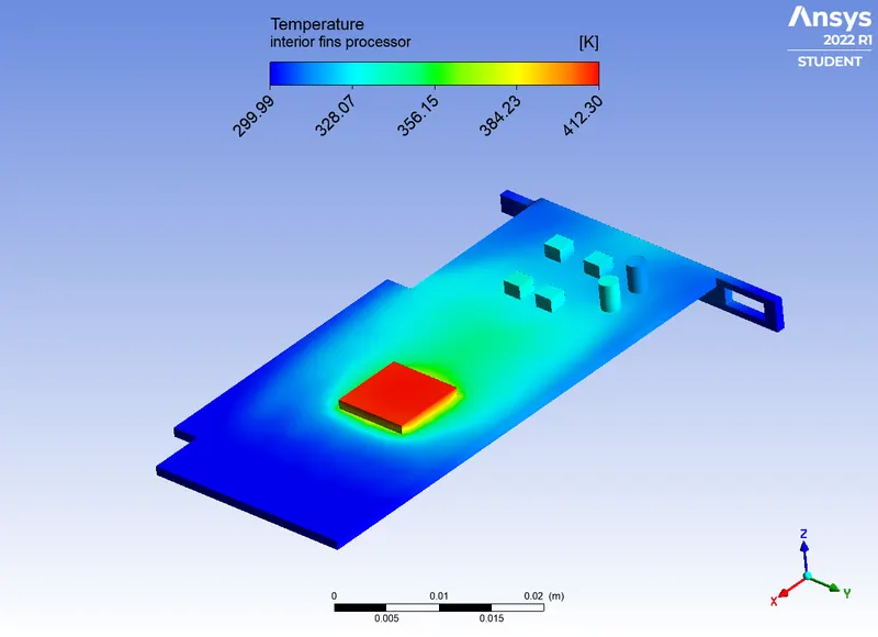
• Temperature hot spots

With Fins

Without Fins

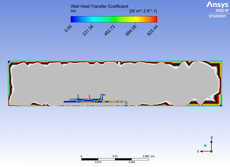
• Wall Heat Transfer Coefficient on plane y =-0.0015m

Inlet velocity of 2.5m/s

• Residuals vs number of iterations

• Temperature monitor vs number of iterations

• Steady state velocity contour on plane y = -0.0015 m

• Temperature hot spots

With Fins

Without Fins

• Wall Heat Transfer Coefficient on plane y =-0.0015m

Inlet velocity of 1m/s

• Residuals vs number of iterations

• Temperature monitor vs number of iterations

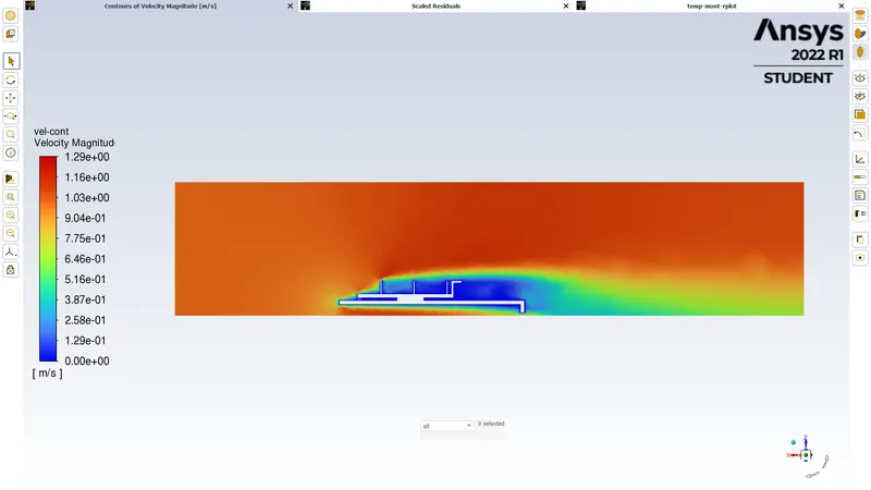
• Steady state velocity contour on plane y = -0.0015 m

• Temperature hot spots

With Fins

Without Fins

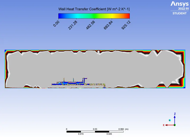
• Wall Heat Transfer Coefficient on plane y =-0.0015m

Conclusions:

From the above plots and contours we note the following observations and conclusions:

1. Residuals do not provide information on the convergence to the steady state of the flow.
2. The temperature monitor for all the three cases reach a steady state value and proves to be a great indicator of the convergence of the steady state problem.
3. As the velocity decreases, we observe that the thermal hot-spots are much stronger in magnitude and have an impact on larger regions of the graphic car. This observation is inline with the theoritical expectation of the effects of the convective heat transfer.
4. The heat transfer coefficient near the fins is highest for inlet velocity of 5m/s. This observation is inline with the experimental trend.