Week 3 - Solving second order ODEs

AIM : Write a program in Matlab that will simulate the pendulum motion.

Theory : Basically, a simple pendulum is a mechanical device demonstrating periodic motion. This has a small circular bob suspended by a thin inextensible string from any fixed end and has length L. It performs oscillatory motion, which is driven by gravitational pull and occurs in the vertical plane.

Examples of simple pendulums are found in clocks, swing sets, and even the natural mechanics of swinging legs.

CODDING :

b=damping coefficient.

m = mass of the ball in kg,

g = gravity in m/s2,

L = length of the pendulum in m,

clear all
close all
clc

b = 0.05;
g = 9.81;
l = 1;
m = 1;

% initial condition
theta_0 = [0;5];

% time points
t_span = linspace(0,10,500)

%solve ODE
[t,results] = ode45(@(t,theta) ode_func(t,theta,b,g,l,m),t_span,theta_0);
plot(t,results(:,1))
hold on
plot(t,results(:,2))
ylabel('plot')
xlabel('time')

if we put this code then a plot will appear and the plot is look like this

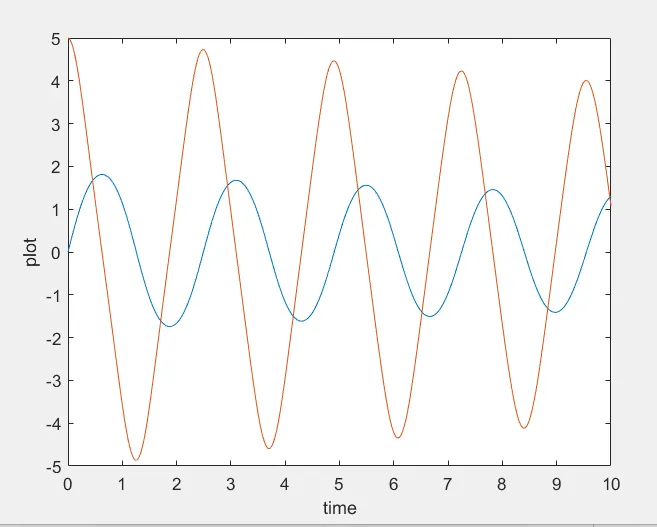
to creat this plot i was getting some error. then i recover error with the helpof our system engineer.

But this is not the end. After doing this i have to create a pendulum so that i have to use more things to create this these are given below.

clear all
close all
clc

b = 0.05;
g = 9.81;
l = 1;
m = 1;

% initial condition
theta_0 = [0;5];

% time points
t_span = linspace(0,10,500)

%solve ODE
[t,results] = ode45(@(t,theta) ode_func(t,theta,b,g,l,m),t_span,theta_0);
plot(t,results(:,1))
hold on
plot(t,results(:,2))
ylabel('plot')
xlabel('time')
hold off

x0 = 0
y0 = 0
% x1 = l1sin_theta
% y1 = -l1costheta

for i = 1 : length(t_span)
    figure(2)
    x1 = l*sin(results(i,1))
   y1 = -l*cos(results(i,1))
   
hold on
plot(x1, y1, 'o', 'MarkerSize', 32);
end

if we put this value then the plot look like this.

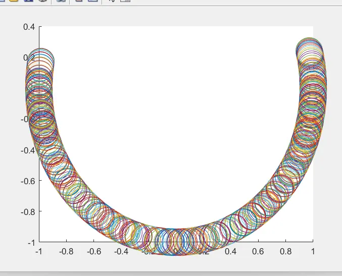
here is the link from where you can check the movement of pendulum.

LINK : https://drive.google.com/file/d/1MU522J7c2-HLWOhKc8ssoqAD4C7dmeK9/view?usp=sharing

thats all

thank you.