Week 6 - CHT Analysis on a Graphics card
AIM:- The project aim is to perform the steady-state conjugate heat transfer analysis on a model of a graphics card.
OBJECTIVE:- The project objectives are-
- Simulate by varying the velocity from 1m/sec to 5m/sec for at least 3 velocities and discuss the results.
- Find out the maximum temperature and heat transfer coefficient attained by the processor.
- Prove that the simulation has achieved convergence with appropriate images and plots.
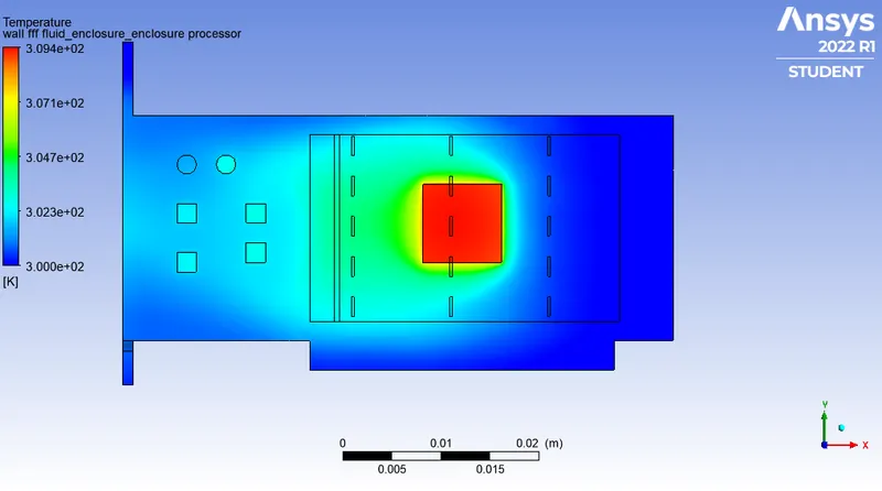
- Identify potential hotspots on the model.
PROJECT DESCRIPTION:-
Conjugate heat transfer corresponds with the combination of heat transfer in solids and heat transfer in fluids. In solids, conduction often dominates whereas, in fluids, convection usually dominates. Conjugate heat transfer is observed in many situations. For example, heat sinks are optimized to combine heat transfer by conduction in the heat sink with the convection in the surrounding fluid.
Common applications and the use cases of this thermal simulation type include electronics cooling, heat exchangers, industrial machinery, some AEC cases, and more.
Heat transfer in solids and heat transfer in fluids are combined in the majority of applications. This is because fluids flow around solids or between solid walls and because solids are usually immersed in a fluid. An accurate description of heat transfer modes, material properties, flow regimes, and geometrical configurations enables the analysis of temperature fields and heat transfer. Such a description is also the starting point for a numerical simulation that can be used to predict conjugate heat transfer effects or to test different configurations in order, for example, to improve the thermal performances of a given application.
Fluid Solid Interaction:-
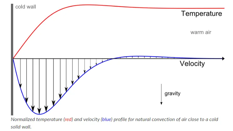
The temperature field and the heat flux are continuous at the fluid/solid interface. However, the temperature field can rapidly vary in a fluid in motion: close to the solid, the fluid temperature is close to the solid temperature, and far from the interface, the fluid temperature is close to the inlet or ambient fluid temperature. The distance where the fluid temperature varies from the solid temperature to the fluid bulk temperature is called the thermal boundary layer.
The thermal boundary layer size and the momentum boundary layer relative size are reflected by the Prandtl number(`Pr = (μ*C_p)/k`) for the Prandtl number to equal 1, thermal and momentum boundary layer thicknesses need to be the same. A thicker momentum layer would result in a Prandtl number larger than 1. Conversely, a Prandtl number smaller than 1 would indicate that the momentum boundary layer is thinner than the thermal boundary layer. The Prandtl number for air at atmospheric pressure and 20°C is 0.7. That is because, for air, the momentum and thermal boundary layer have similar sizes, while the momentum boundary layer is slightly thinner than the thermal boundary layer. For water at 20°C, the Prandtl number is about 7. So, in water, the temperature changes close to a wall are sharper than the velocity change.
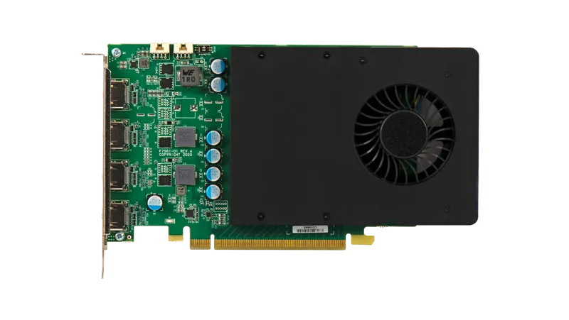
In electronics equipement, instrumentation, and computers, electronic components, such as intregated circuits, resistors, transistors, diodes, and capacitors, are soldered onto Printed Circuit Boards(PCBs). The PCBs are often stacked in rows. Because many of these electronic components must dissipate heat, cooling air is often blown through the air gap between each pair of PCBs to keep the components from getting too hot. The graphic card is the main component which is responsible for the better quality of the visuals displayed. In this experiment we study the maximum temperature and heat transfer coefficient attained by the processor with effect of different inlet velocities.
We perform the simulation in different velocity from 1m/s to 5m/s. So, we take three values of velocity which are 1m/s, 3m/s and 5m/s and now we ready to go for our next step. Before jump into our project, we devide our simulation into two parts. In first case, we just take a normal mesh size for whole geometry including our enclosure which is mainly a fluid region. And in our second case, we refined our geometry basically we juse increase the number of elements of the Graphics card only which we discuss in later.
CASE-1:-
We jus devide our simulation process into three parts
- Preprocessing and Mesh
- Case Setup
- Postprocessing Results
Preprocessing and Mesh:-
Geometry:-
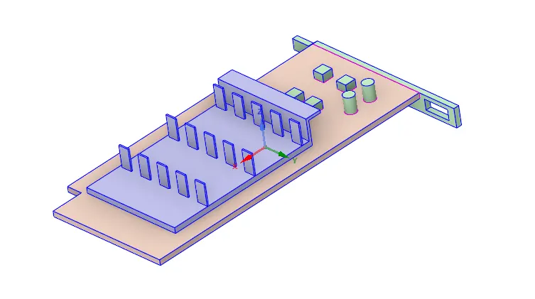
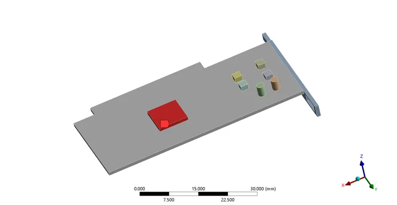
Graphics card model which we use to simulate
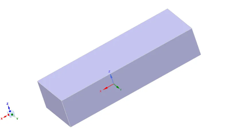
The enclosure is created mainly for creating a fluid region. After creating an enclosure we need to turn on the shared topology where our solid body shares the information with our fluid region.
Mesh:-
Base Mesh is created where I take 2mm element size for whole geometry-
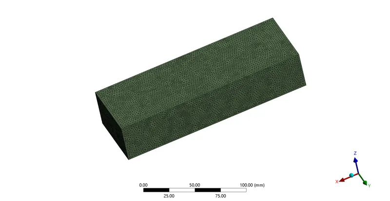
After generating mesh, the graphics card looks like-
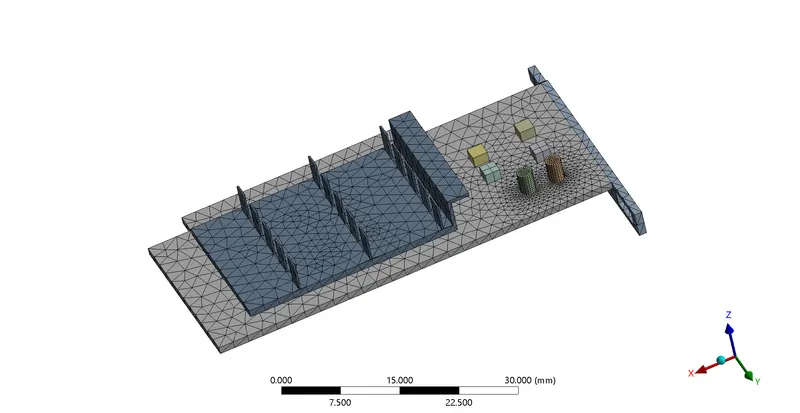
Mesh Details:-
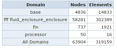
Now, we can go for Name selection process.
Name Selection Process:-
Inlet:- I select one side as inlet which is closest to our model.
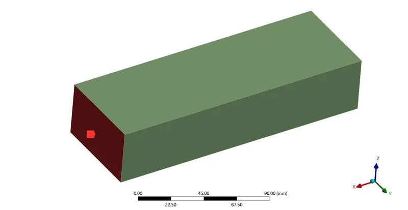
Outlet:- Another side I select as outlet.
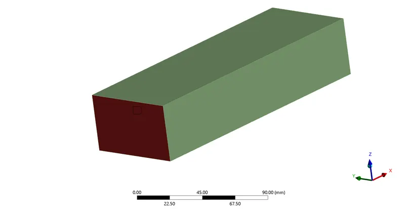
Symmetry:- Three side of enclosure I select as symmetry.
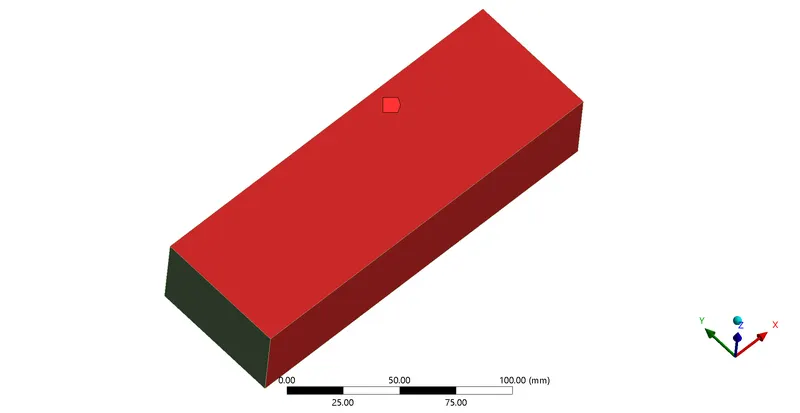
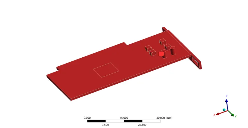
Wall:- One side of the enclosure we select as the wall is the below side of our graphic card model.
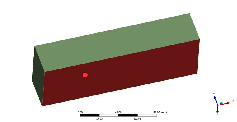
Fin:-
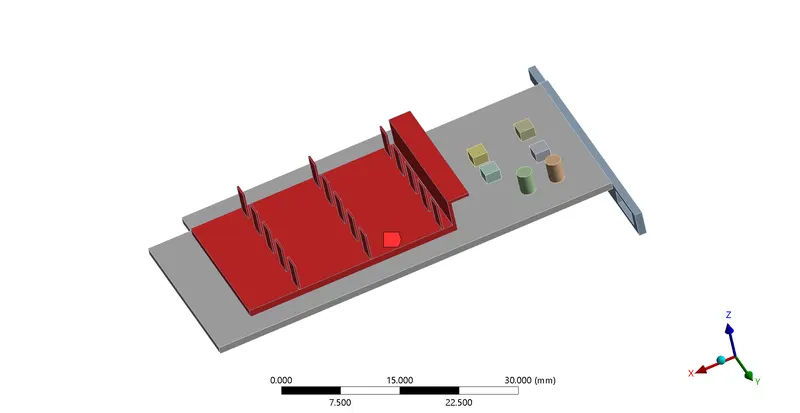
Processor:-
Base:-
Case Setup:-
- Pressure-based solver and Absolute velocity are used.
- Steady-state simulation is performed
- The standard k-epsilon turbulence model is taken as a viscous model.
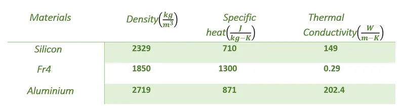
- In the simulation, 3 materials are taken as solid. The first one is Fr4 which is a class of printed circuit board base material made from a flame retardant epoxy resin and glass fabric composite and it has poor thermal conductivity. The second one is Aluminium which is taken as Fin material from where most of the heat transfer takes place. And the third one is silicon which is taken as Processor material from where heat is generated. And the air is taken as fluid.
- Solid Material specifications are-
-
We assume here only the processor is a source of heat energy and consider that its power is 1W. We need to calculate the amount of generated heat by the processor, so
Generated heat = `P/V`
Where P is the power and V is the processor’s volume.
Processor Volume = `8 xx 8 xx 1` = 64 `mm^3` = `64 xx 10^-9 m^3`
So, Generated heat = `P/V = 1/(64 xx 10^-9) W/m^3` = 15625000 W/m^3
- In Pressure velocity coupling, a Coupled scheme is used.
Here is the report for the whole simulation, we can see all the values which we take to simulate our graphics card model. This is a report for the velocity of 1m/s.
Fluent
Version: 3d, dp, pbns, ske (3d, double precision, pressure-based, standard k-epsilon)
Release: 22.1.0
Title:


Models
------

   Model                        Settings
   ----------------------------------------------------------------
   Space                        3D
   Time                         Steady
   Viscous                      Standard k-epsilon turbulence model
   Wall Treatment               Standard Wall Functions
   Heat Transfer                Enabled
   Solidification and Melting   Disabled
   Radiation                    None
   Species                      Disabled
   Coupled Dispersed Phase      Disabled
   NOx Pollutants               Disabled
   SOx Pollutants               Disabled
   Soot                         Disabled
   Mercury Pollutants           Disabled
   Structure                    Disabled
   Acoustics                    Disabled
   Eulerian Wall Film           Disabled
   Potential/Li-ion Battery     Disabled
   Multiphase                   Disabled


Material Properties
-------------------

   Material: fr4 (solid)

      Property               Units      Method     Value(s)
      -----------------------------------------------------
      Density                kg/m^3     constant   1850
      Cp (Specific Heat)     J/(kg K)   constant   1300
      Thermal Conductivity   W/(m K)    constant   0.29

   Material: silicon (solid)

      Property               Units      Method     Value(s)
      -----------------------------------------------------
      Density                kg/m^3     constant   2329
      Cp (Specific Heat)     J/(kg K)   constant   710
      Thermal Conductivity   W/(m K)    constant   149

   Material: air (fluid)

      Property                        Units      Method     Value(s)
      ----------------------------------------------------------------
      Density                         kg/m^3     constant   1.225
      Cp (Specific Heat)              J/(kg K)   constant   1006.43
      Thermal Conductivity            W/(m K)    constant   0.0242
      Viscosity                       kg/(m s)   constant   1.7894e-05
      Molecular Weight                kg/kmol    constant   28.966
      Thermal Expansion Coefficient   K^-1       constant   0
      Speed of Sound                  m/s        none       #f

   Material: aluminum (solid)

      Property               Units      Method     Value(s)
      -----------------------------------------------------
      Density                kg/m^3     constant   2719
      Cp (Specific Heat)     J/(kg K)   constant   871
      Thermal Conductivity   W/(m K)    constant   202.4


Cell Zone Conditions
--------------------

   Zones

      name                            id   type
      ------------------------------------------
      fff-fluid_enclosure_enclosure   10   fluid
      fin                             13   solid
      processor                       14   solid
      base                            15   solid

   Setup Conditions

      fff-fluid_enclosure_enclosure

         Condition       Value
         ---------------------
         Frame Motion?   no

      fin

         Condition       Value
         ------------------------
         Material Name   aluminum
         Frame Motion?   no

      processor

         Condition               Value
         --------------------------------------------------------------------------------------
         Material Name           silicon
         Specify source terms?   yes
         Source Terms            ((energy ((constant . 15625000) (inactive . #f) (profile  ))))
         Frame Motion?           no

      base

         Condition       Value
         ---------------------
         Frame Motion?   no


Boundary Conditions
-------------------

   Zones

      name                                                  id   type
      --------------------------------------------------------------------------
      wall-base-fff-fluid_enclosure_enclosure               1    wall
      wall-fff-fluid_enclosure_enclosure-processor          3    wall
      wall-fff-fluid_enclosure_enclosure-fin                4    wall
      inlet                                                 16   velocity-inlet
      outlet                                                17   pressure-outlet
      wall                                                  18   wall
      symmetry                                              19   symmetry
      wall-fff-fluid_enclosure_enclosure-fin-shadow         12   wall
      wall-fff-fluid_enclosure_enclosure-processor-shadow   20   wall
      wall-base-fff-fluid_enclosure_enclosure-shadow        21   wall

   Setup Conditions

      wall-base-fff-fluid_enclosure_enclosure

         Condition                  Value
         ------------------------------------------
         Material Name              aluminum
         Thermal BC Type            Coupled
         Wall Motion                Stationary Wall
         Shear Boundary Condition   No Slip

      wall-fff-fluid_enclosure_enclosure-processor

         Condition         Value
         --------------------------
         Material Name     aluminum
         Thermal BC Type   Coupled

      wall-fff-fluid_enclosure_enclosure-fin

         Condition                  Value
         ------------------------------------------
         Material Name              aluminum
         Thermal BC Type            Coupled
         Wall Motion                Stationary Wall
         Shear Boundary Condition   No Slip

      inlet

         Condition                  Value
         --------------------------------
         Velocity Magnitude [m/s]   1

      outlet

         Condition   Value
         -----------------

      wall

         Condition                  Value
         ------------------------------------------
         Material Name              aluminum
         Thermal BC Type            Heat Flux
         Wall Motion                Stationary Wall
         Shear Boundary Condition   No Slip

      symmetry

         Condition   Value
         -----------------

      wall-fff-fluid_enclosure_enclosure-fin-shadow

         Condition         Value
         --------------------------
         Material Name     aluminum
         Thermal BC Type   Coupled

      wall-fff-fluid_enclosure_enclosure-processor-shadow

         Condition                  Value
         ------------------------------------------
         Material Name              aluminum
         Thermal BC Type            Coupled
         Wall Motion                Stationary Wall
         Shear Boundary Condition   No Slip

      wall-base-fff-fluid_enclosure_enclosure-shadow

         Condition         Value
         --------------------------
         Material Name     aluminum
         Thermal BC Type   Coupled


Solver Settings
---------------

   Equations

      Equation     Solved
      -------------------
      Flow         yes
      Turbulence   yes
      Energy       yes

   Numerics

      Numeric                         Enabled
      ---------------------------------------
      Absolute Velocity Formulation   yes

   Pseudo Time Explicit Relaxation Factors

      Variable                     Relaxation Factor
      ----------------------------------------------
      Density                      1
      Body Forces                  1
      Turbulent Kinetic Energy     0.75
      Turbulent Dissipation Rate   0.75
      Turbulent Viscosity          1
      Energy                       0.75
      Explicit Momentum            0.5
      Explicit Pressure            0.5

   Linear Solver

      Variable                     Solver Type   Termination Criterion   Residual Reduction Tolerance
      -----------------------------------------------------------------------------------------------
      Flow                         F-Cycle       0.1
      Turbulent Kinetic Energy     F-Cycle       0.1
      Turbulent Dissipation Rate   F-Cycle       0.1
      Energy                       F-Cycle       0.1

   Pressure-Velocity Coupling

      Parameter                               Value
      -----------------------------------------------
      Type                                    Coupled
      Pseudo Time Method (Global Time Step)   yes

   Discretization Scheme

      Variable                     Scheme
      ------------------------------------------------
      Pressure                     Second Order
      Momentum                     Second Order Upwind
      Turbulent Kinetic Energy     First Order Upwind
      Turbulent Dissipation Rate   First Order Upwind
      Energy                       Second Order Upwind

   Solution Limits

      Quantity                         Limit
      ---------------------------------------
      Minimum Absolute Pressure        1
      Maximum Absolute Pressure        5e+10
      Minimum Temperature              1
      Maximum Temperature              5000
      Minimum Turb. Kinetic Energy     1e-14
      Minimum Turb. Dissipation Rate   1e-20
      Maximum Turb. Viscosity Ratio    100000
Postprocessing Results:-
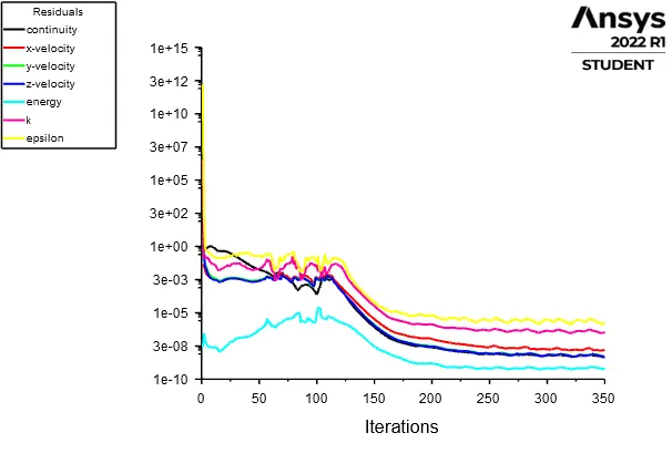
Residual:-
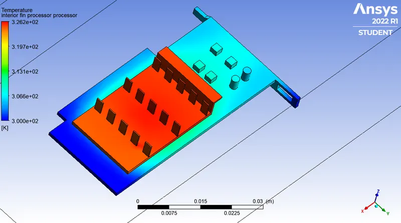
Temperature Contour:-
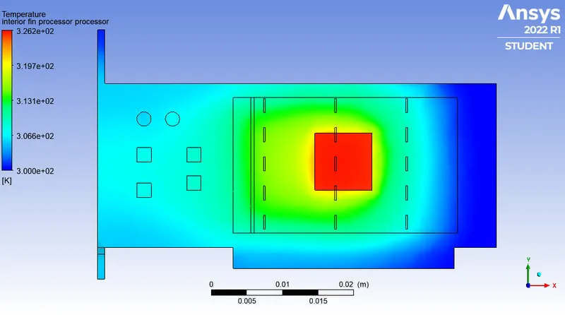
Global Hotspot region:-
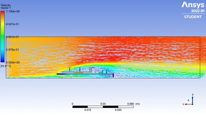
Velocity Vector:-
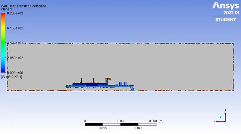
Wall Heat Transfer Coefficient:-
For the other two velocities the Preprocessing, Mesh, and Case setup are the same so we just focus on the post-processing results.
Postprocessing Results For 3m/s and 5m/s :-
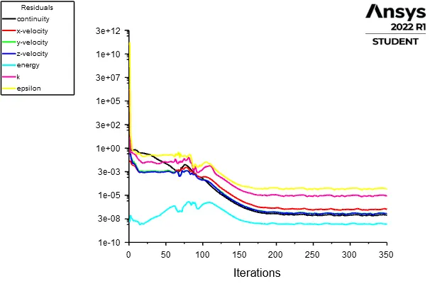
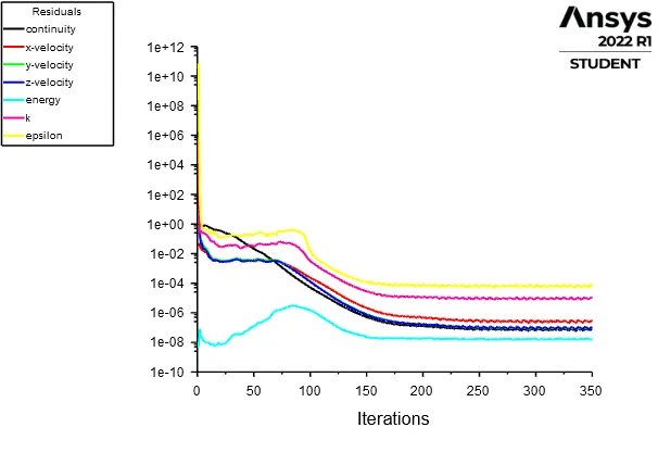
Residual for 3m/s and 5m/s respectively:-
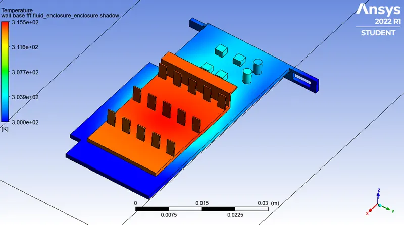
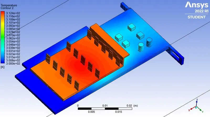
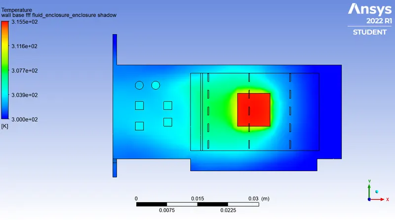
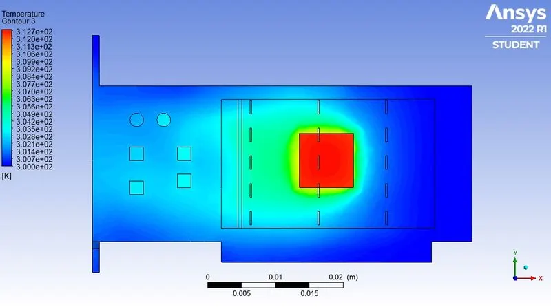
Temperature Contour for 3m/s and 5m/s respectively:-
Global Hotspot region for two velocities:-
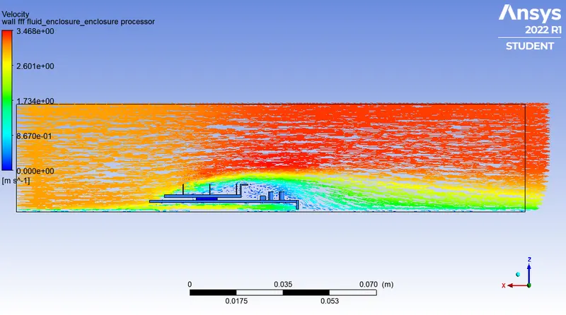
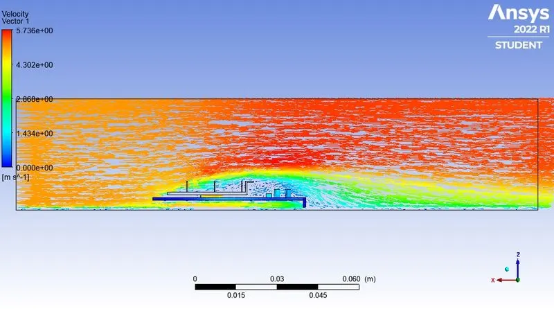
Velocity Vector for two velocities:-
Wall Heat Transfer Coefficient for two velocities:-
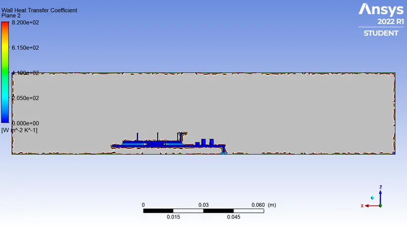
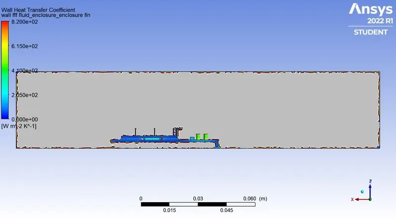
So, the results we get from our simulation is-
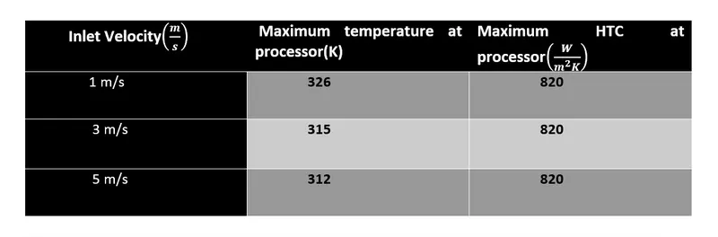
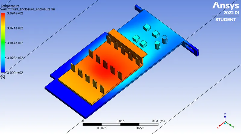
So we can see that for the higher velocity we get a lower temperature. That's why in case_2, we take a velocity of 5 m/s for our simulation to see is there any difference in the result.
CASE-2:-
In case_2, all the processes are the same as previously we have done. Here we just refined our mesh means we increase the mesh elements of our geometry by specifying the mesh element size of each body instead of taking uniform element size for the whole geometry.
Mesh details:-
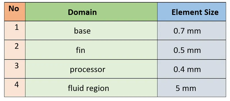
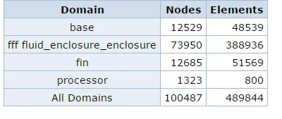
After meshig our geometry looks like -
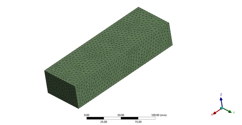
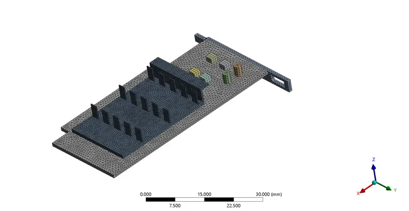
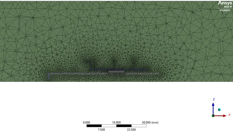
As we mentioned previously that all other processes like case setup same as previous, so we jump into the Postprocessing results.
Postprocessing Results:-
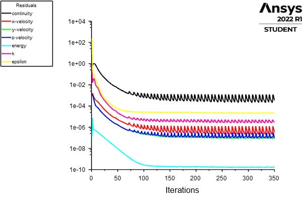
Residuals:-
Temperature Contour:-
Global Hotspot Region:-
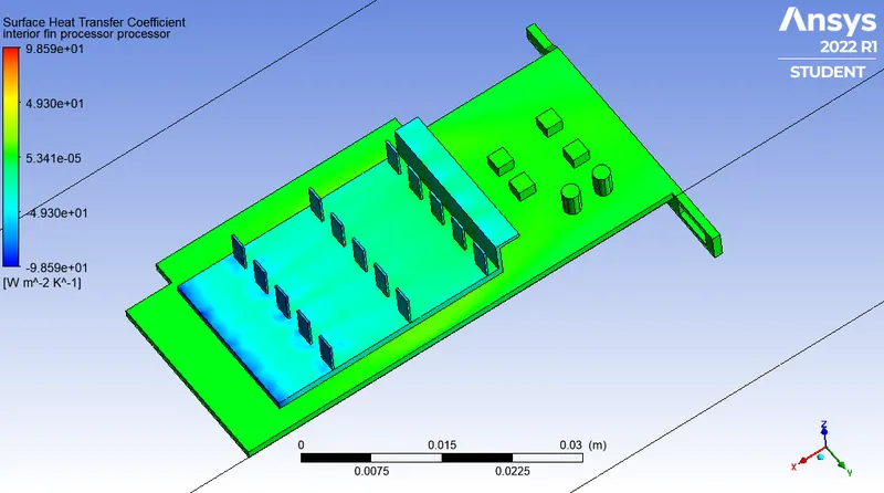
Surface Heat transfer Coefficient:-
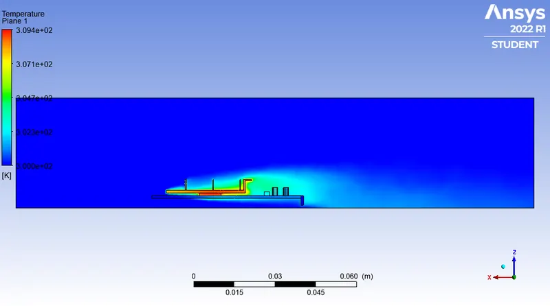
Temperature Plot:-
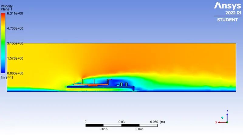
Velocity Plot:-
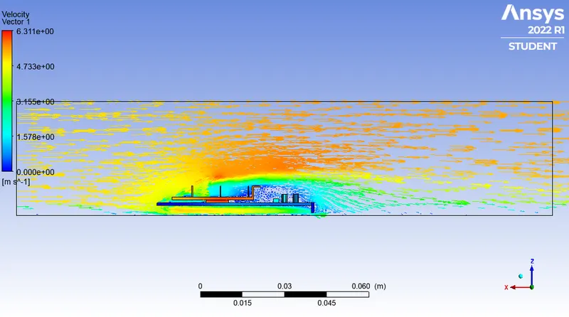
Velocity Vector:-
Wall Heat Transfer Coefficient:-
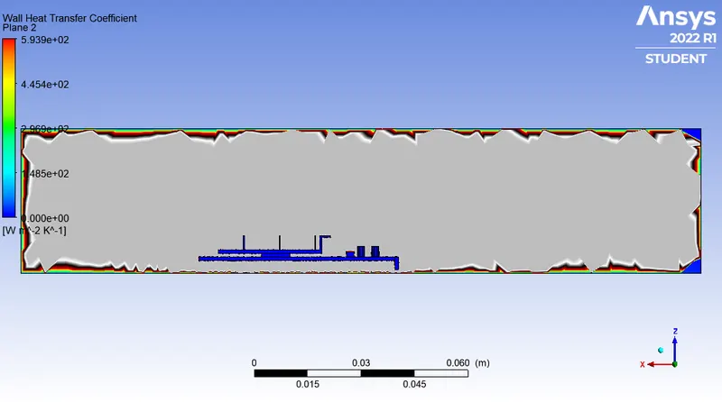
So, in the case of 5 m/s velocity, the value of the maximum temperature of the processor and maximum heat transfer coefficient for both the coarse and refined mesh are
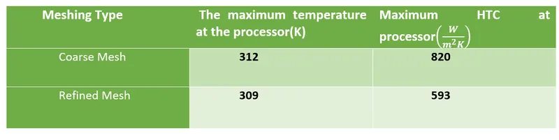
We can see here in a refined case we get more optimum results. More refined means more accurate results, but also more refined means more time is required to converge. So, we can refine a mesh up to a level from where we get a more accurate result in a lesser time.
If we see our residual plots after a certain iteration, it's not dropping. These plots are going in a straight line which means our simulation has achieved convergence.
CONCLUSION:-
- A Graphics card is a very necessary component in many electronic devices which is responsible for the better quality of the visuals displayed. And with that, it also generates lots of heat and it is necessary to flow cool air on it to keep it from getting too hot.
- For better cooling of the graphics card, cooling air velocity needs to be higher because it helps to keep the graphics card at a lesser temperature.
- By seeing the residual plots, we can conclude that our simulation has fully converged.
- Refined mesh gives optimum results but it takes more time.