Week 6 - CHT Analysis on a Graphics card

Conjugate Heat-Transfer Analysis on a Graphics card

CHT analysis:-

The Conjugate Heat Transfer (CHT) analysis type allows for the simulation of heat transfer between solid and fluid domains by exchanging thermal energy at the interfaces between them.

Applications:

• simulation of heat exchangers.
• cooling of electronic equipment.
• general-purpose cooling and heating systems.

Procedure:

1. Geometry
2. Meshing
3. Setup
4. Solution
5. Results

Open Ansys Workbench and create Fluent as a standalone system.

----------------------------------------------------------------------------------------------------------------------

1.Geometry Preparation:-

• Import the given graphics card file.
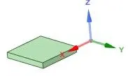
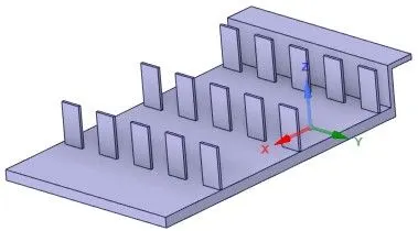
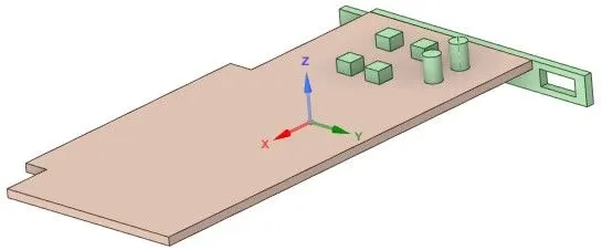
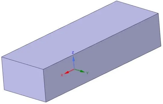
• Key components are Processor, Fins, Base, Enclosure.
• Processor:-
• 
• Fins:-
• 
• Base:-
• 
• Enclosure:-
• 
• 
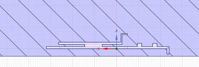
• Combined view:-
• 
• 
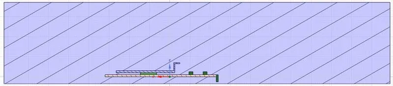
• At this stage Topology between solid and fluid domains has not been shared.
• So we have to share the Topology so that solution information gets shared in between those bodies.
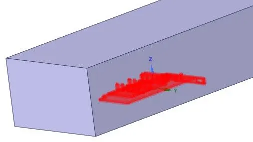
• Workbench => Share => Topology shared.
• 

----------------------------------------------------------------------------------------------------------------------

2. Meshing:-

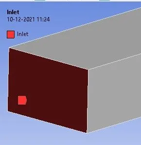
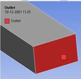
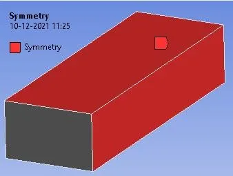
• Creating Named sections
  • 

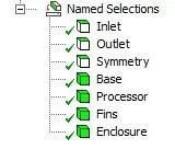
Inlet:-

Outlet:-

Symmetry (outer faces of enclosure):-

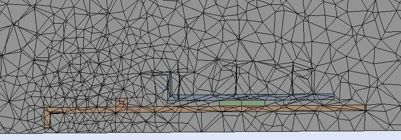
• Global Element size = 5 mm
• Base & fins Element size = 2 mm
• Processor element size = 1 mm
• Elements = 115427; Nodes = 20675.
• 
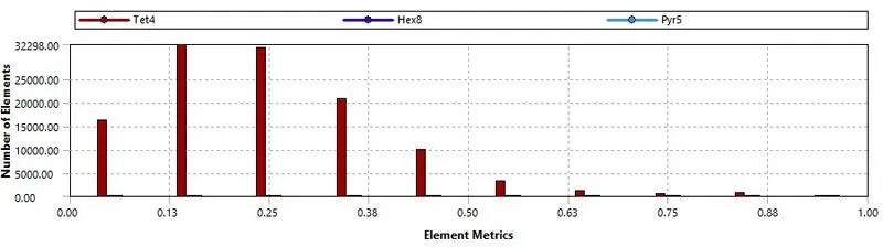
• Skewness:-
• 
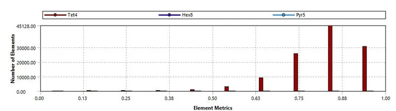
• Element quality:-
• 

----------------------------------------------------------------------------------------------------------------------

3. Setup & solution:-

• Double Presission, Solve processers = 4.
• General
  • Solver = Pressure Based.
  • Velocity Formulation = Absolute.
  • Time= Steady
• Models:
  • Energy = on
  • Viscous Model = k-epsilon.
    • Model = Realizable.
    • Near-wall Treatment = Enhanced wall Treatment.
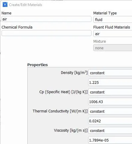
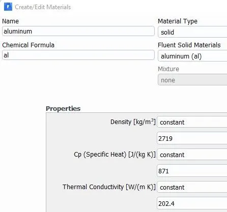
• Materials:-
• Fluids = Air
• 
• Solids = Aluminium, Copper, Silicon
• 
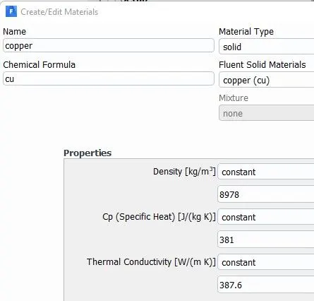
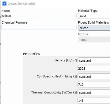
• Cell Zone conditions:-
  • Enclosure = fluid => air
  • Processor = Solid => Copper
  • Fins = Solid => Aluminium
  • Base = Solid => Silicon
• Boundary Conditions:-
  • Inlet = Velocity inlet
    • We are solving for 5 different Velocity 1,2,3,4,5 m/s.
    • Temperature = 300 K
  • Outlet = Pressure outlet
    • Guage pressure = 0 Pa
• Residual Monitors:
  • Uncheck the convergence for all equations.
• Initialization:
  • Hybrid Initialization
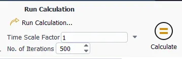
• Run Calculations:-
  • Steady-State Simulation
    • 

----------------------------------------------------------------------------------------------------------------------

4.Results:-

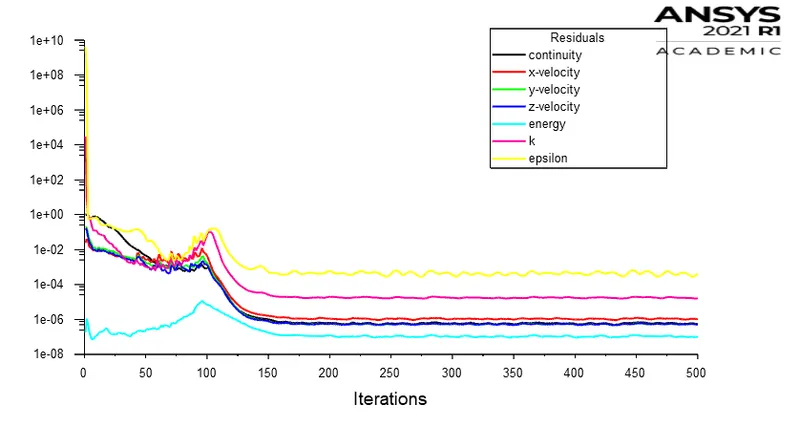
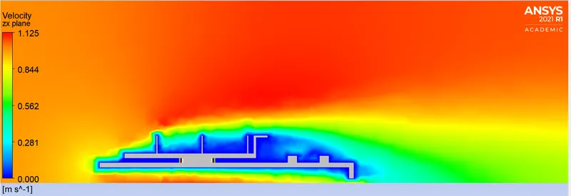
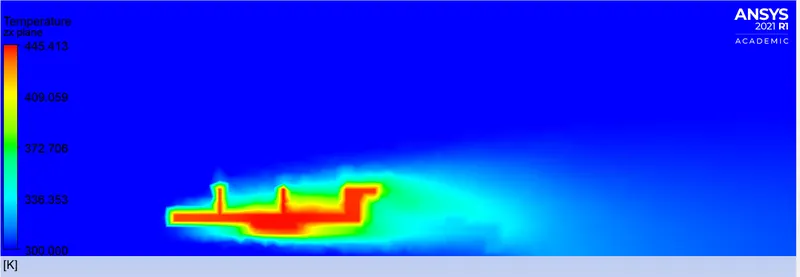
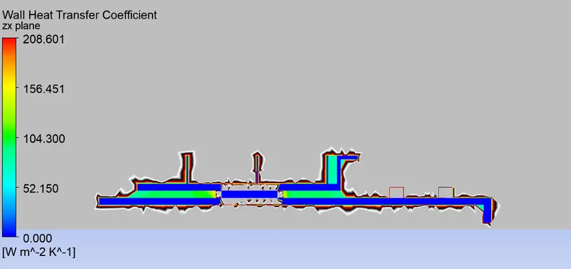
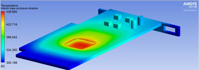
1. Velocity = 1 m/s

Residuals:-

:

Contour Plots:-

Potential Hotspots:-

----------------------------------------------------------------------------------------------------------------------

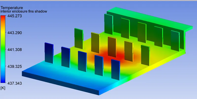
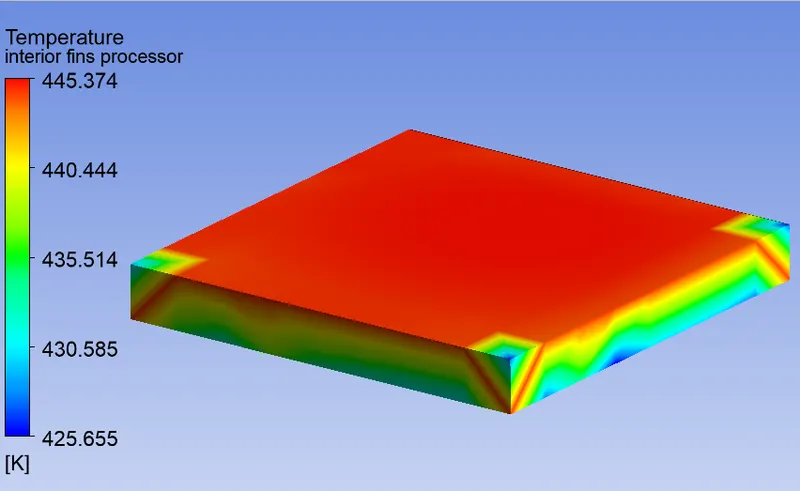
2. Velocity = 2 m/s

Residuals:-

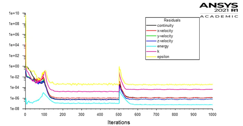
Contour Plots:-

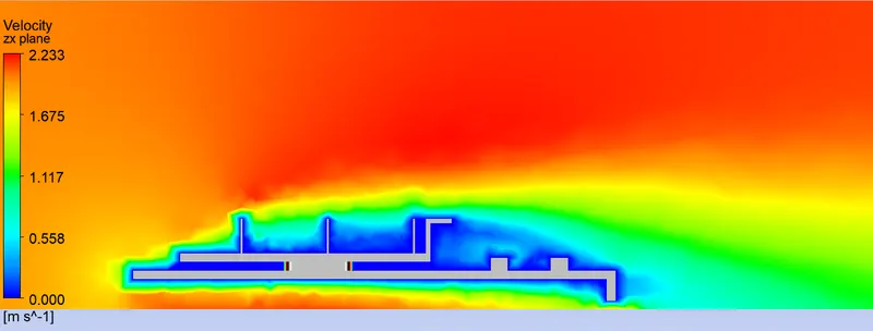
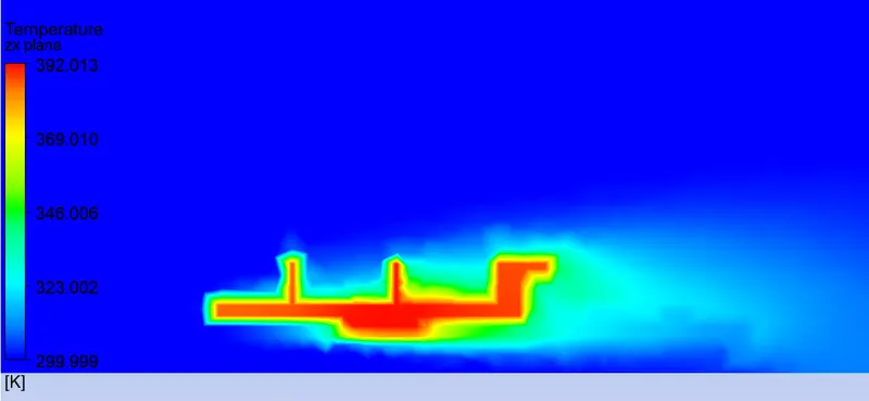
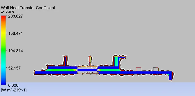
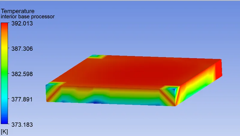
Potential Hotspots:-

----------------------------------------------------------------------------------------------------------------------

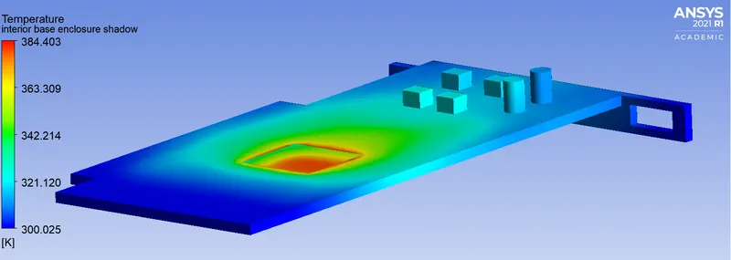
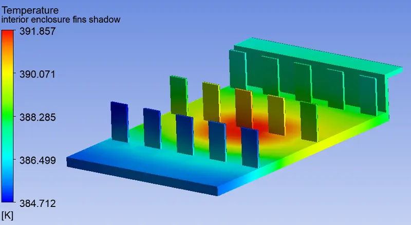
3. Velocity = 3 m/s

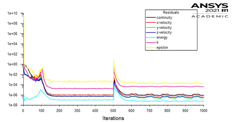
Residuals:-

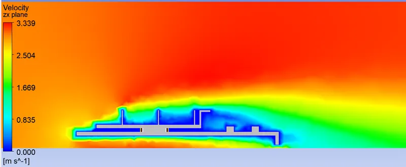
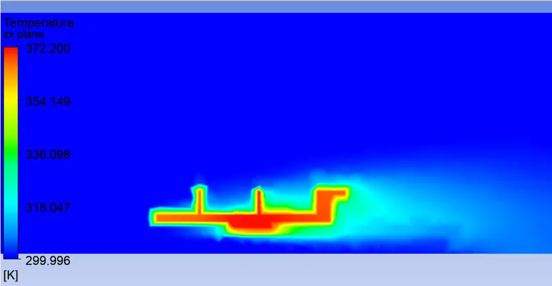
Contour Plots:-

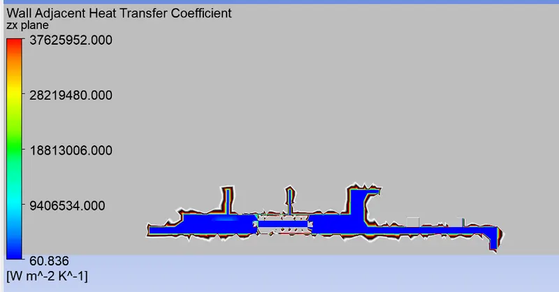
Potential Hotspots:-

----------------------------------------------------------------------------------------------------------------------

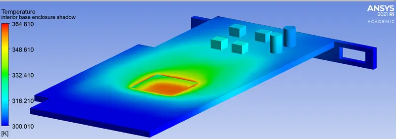
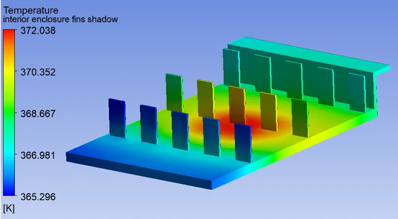
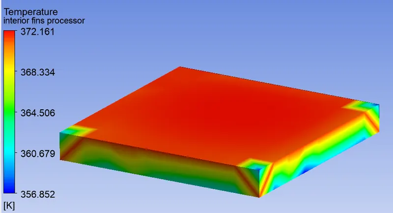
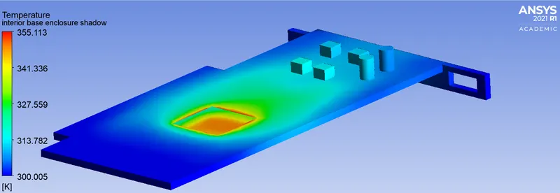
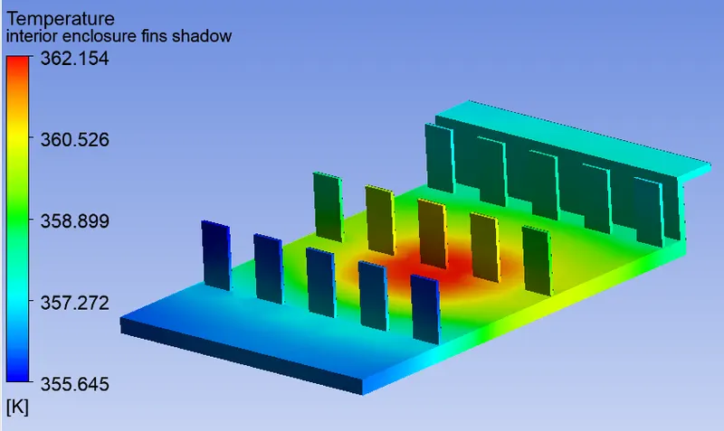
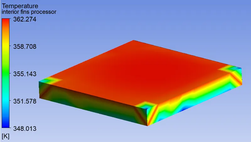
4. Velocity = 4 m/s

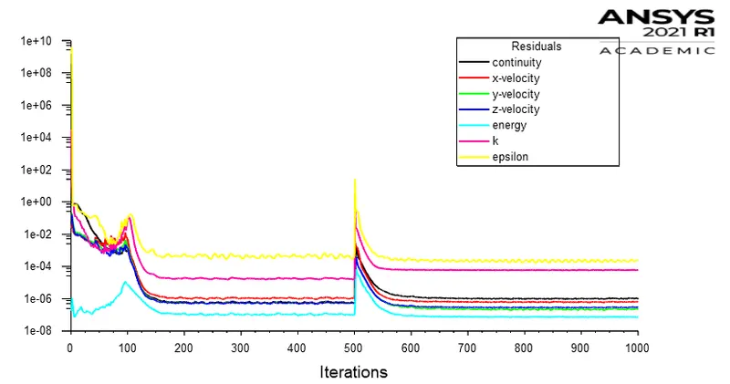
Residuals:-

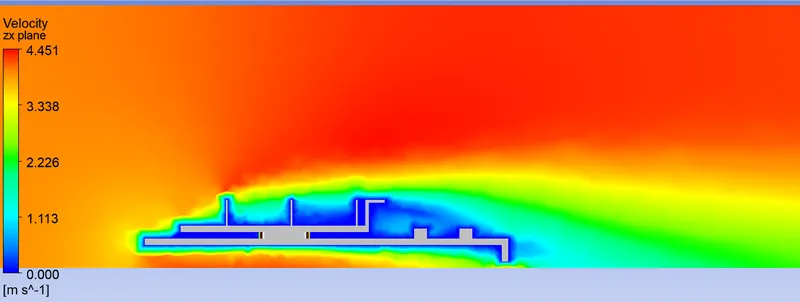
Contour Plots:-

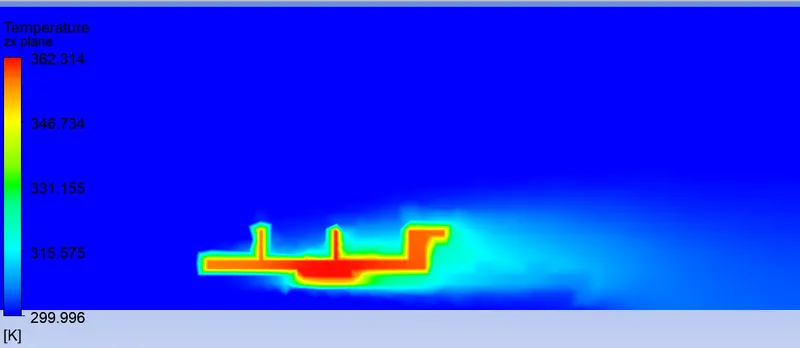
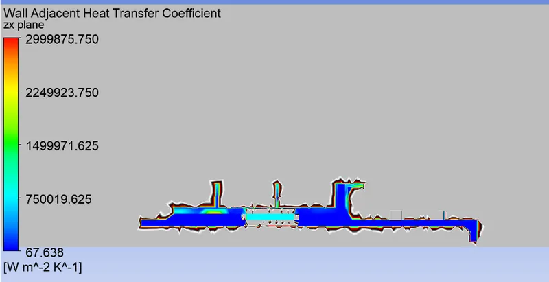
Potential Hotspots:-

----------------------------------------------------------------------------------------------------------------------

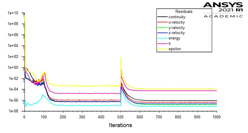
5. Velocity = 5 m/s

Residuals:-

Contour Plots:-

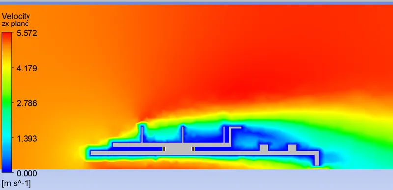
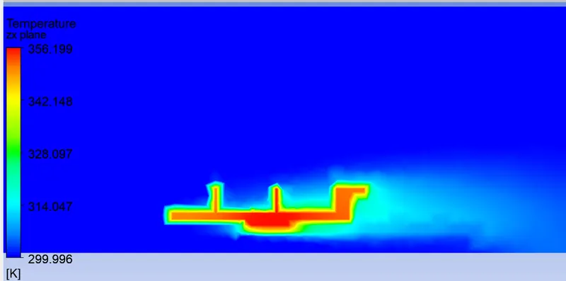
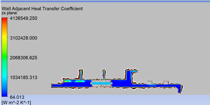
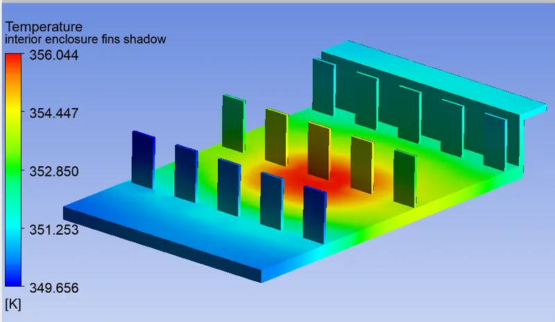
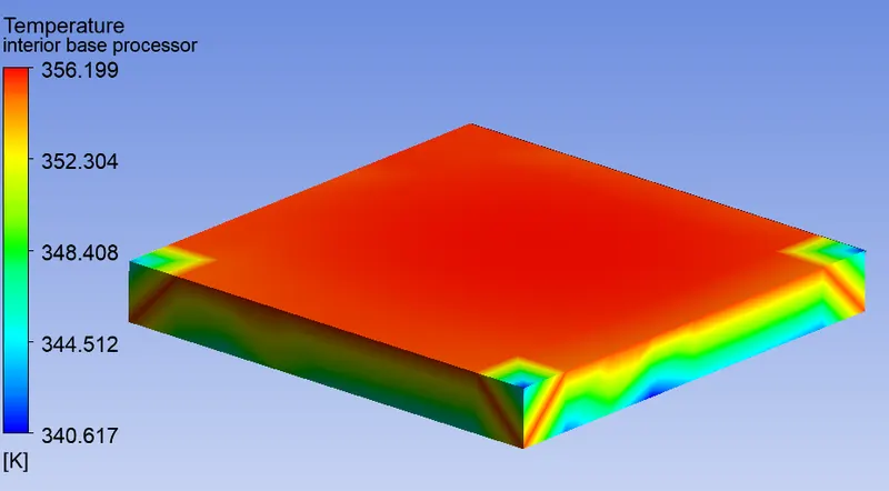
Potential Hotspots:-

---------------------------------------------------------------------------------------------------------------------
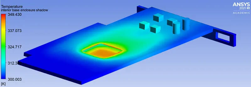