CHT Analysis on a Graphics card
CHT Analysis on a Graphics card
The contemporary conjugate convective heat transfer model was developed after computers came into wide use to substitute the empirical relation of proportionality of heat flux to temperature difference with heat transfer coefficient which was the only tool in theoretical heat convection since the times of Newton. This model, based on a strictly mathematically stated problem, describes the heat transfer between a body and a fluid flowing over or inside it as a result of the interaction of two objects. The physical processes and solutions of the governing equations are considered separately for each object in two subdomains. Matching conditions for these solutions at the interface provide the distributions of temperature and heat flux along the body–flow interface, eliminating the need for a heat transfer coefficient. Moreover, it may be calculated using these data.
The Conjugate Heat Transfer (CHT) analysis type allows for the simulation of heat transfer between solid and fluid domains by exchanging thermal energy at the interfaces between them. Typical applications of this analysis type exist as, but are not limited to, the simulation of heat exchangers, cooling of electronic equipment, and general-purpose cooling and heating systems.
Applications
Conjugate heat transfer problems, where the heat conduction in a solid region is usually coupled with the convection heat transfer in an adjacent fluid region, are of great significance in many practical applications, for example, the electronic circuit cooling, the design of thermal protection system for space vehicles, thermal insulation of nuclear reactor, turbine blade cooling, and solar panel design.
Conjugate Heat Transfer (CHT) is applicable whenever there are two adjacent domains and we wish to analyze the heat transfer between these domains. These domains can either be solid or fluid. One example is the forced or natural convective cooling of a heat-sink attached to active electronics components which generate heat
For many simulations of real-world engineering applications, the predictions of heat transfer properties are as important, if not more important, than the actual flow field. Such scenarios include simulations of heat exchangers, HVAC (Heating, Ventilation and Air Conditioning), combustion/burners, electronics cooling, and many more. In these applications, we are often interested in how heat moves through both the fluid and solid domains, and importantly the transfer of heat across the interface between adjacent domains.
About this project
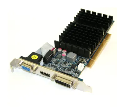
Conjugate heat transfer is a behavioural analysis where convective (transfer between fluid) and conductive (transfer between solids) heat transfer takes place in a system. This combination of heat transfer has forced or natural convection where fluid is dominated by convection and solid is dominated by conduction. The objective of the Experiment is to Carry out mesh Independent study Stimulate CHT using two different processor materials Carry out the analysis at different velocities To determine the hot spots and Heat transfer co-efficient at different velocities
According to NVIDIA, the standard operating temperature of a graphics processing unit (GPU) is 104°F to 194°F (40°C to 90°C). Since room temperature is 68°F (20°C), as defined by the National Institute of Standards and Technology, your GPU will always be and feel warm or hot while operating at any given time.
While ideal GPU temperatures are usually between 65° to 85° Celsius (149° to 185° F) under load, AMD GPUs (like the Radeon RX 5700 or 6000 Series) can safely reach temperatures as high as 110 degrees Celsius (230° F)
The power consumption of today's graphics cards has increased a lot. The top models demand between 110 and 270 watts from the power supply; in fact, a powerful graphics card under full load requires as much power as the rest of the components of a PC system combined.
Our Objectives:
- Simulate by varying the velocity from 1m/sec to 5m/sec for at least 3 velocities
- Find out the maximum temperature and heat transfer coefficient attained by the processor.
- Prove that the simulation has achieved convergence
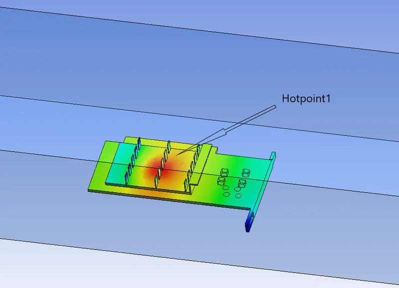
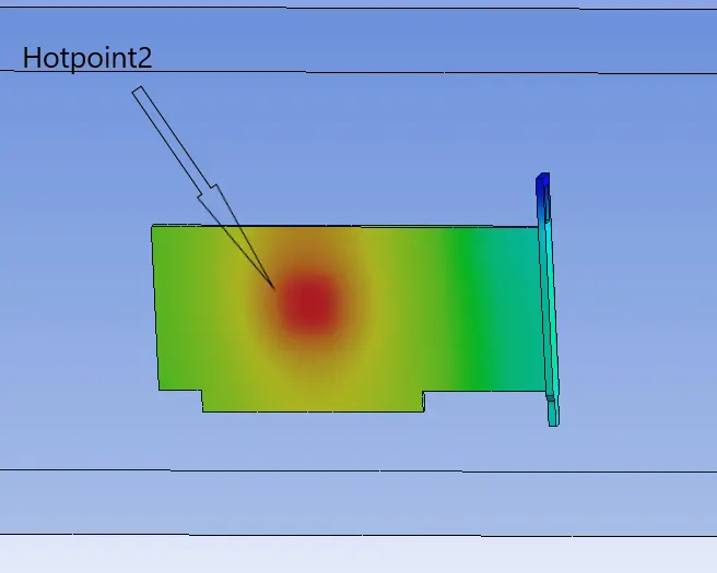
- potential hotspots on the model.
BASELINE MESH
Course mesh without any body sizing and the inlet velocity 3 m/s
Geometry:-
Shared
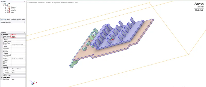
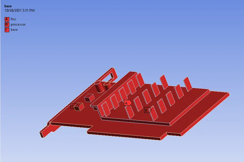
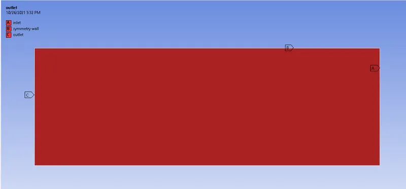
Named selection
Meshing:-
With element size 10 mm
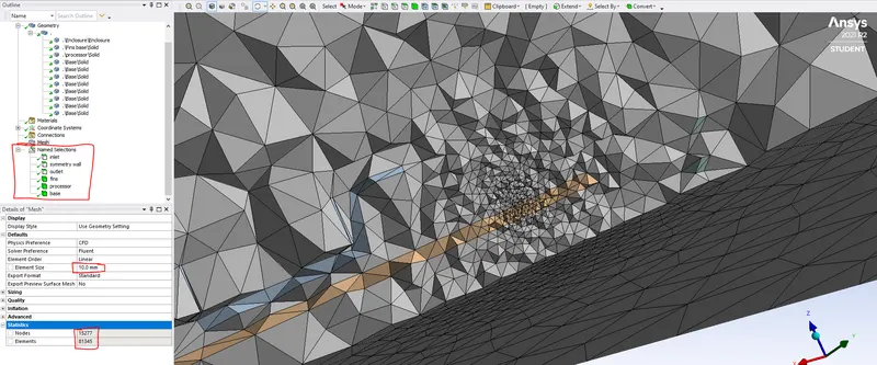
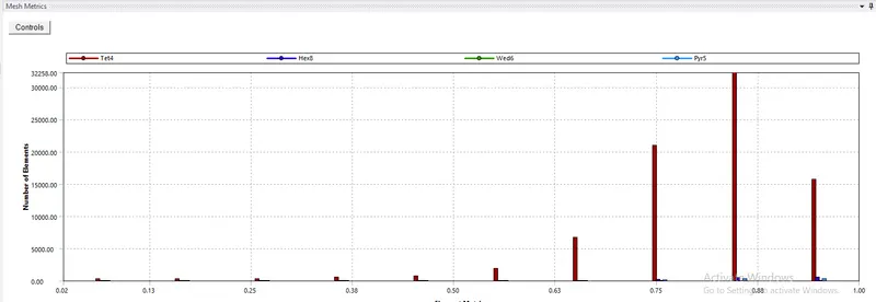

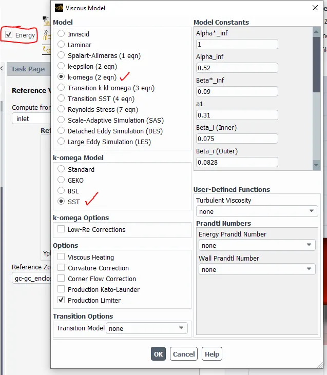
Setup:-
We have to calculate the temperature near the wall which k-Omega is used to calculate near the wall
The default will be air for fluid and aluminium for the solid and we are adding the copper
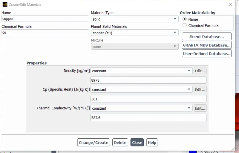
Converting the graphic card parts as solid
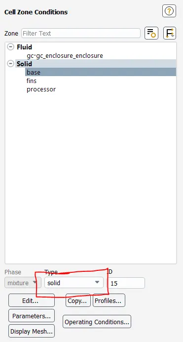
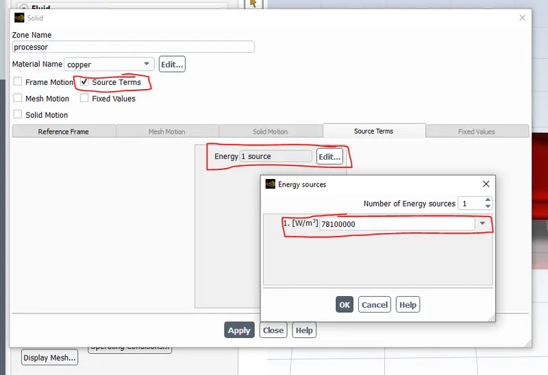
Here the source term is the processor
Assuming 5 watt
Q = Watt/Volume of the processor W/m^3
Q = `5/(64e-9)`
Q = 78100000 W/m^3
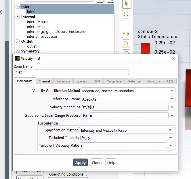
Inlet velocity 3 m/s
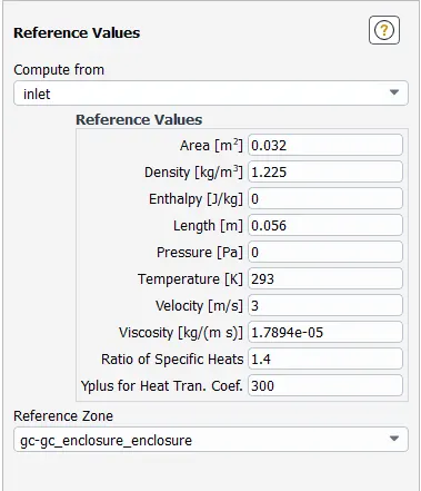
We have given the inlet temperature as 293k
To find out the maximum temperature and heat transfer coefficient attained by the processor
Facet maximum is used to calculate the max value of the variable



Results:-
simulation has achieved convergence
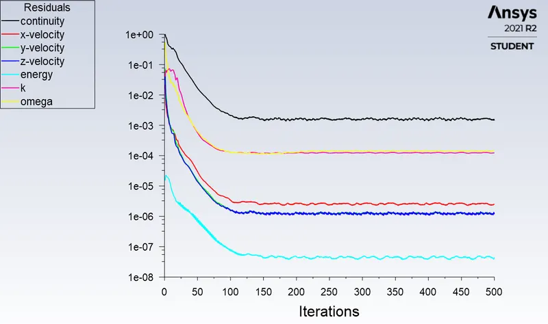
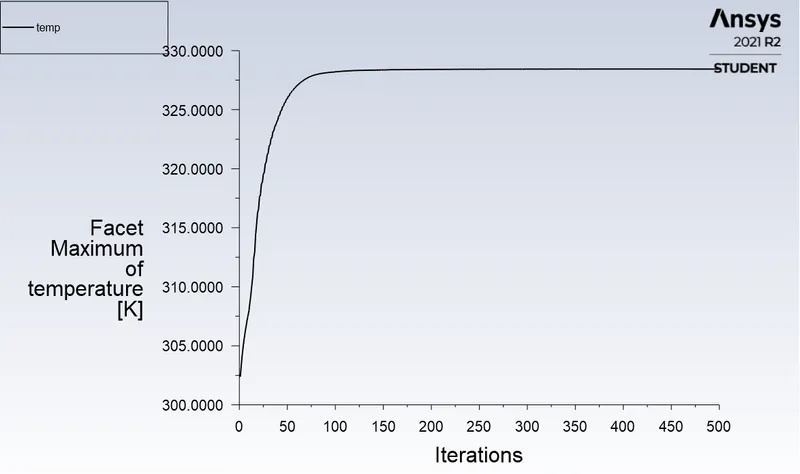
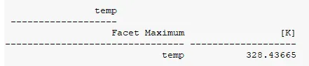
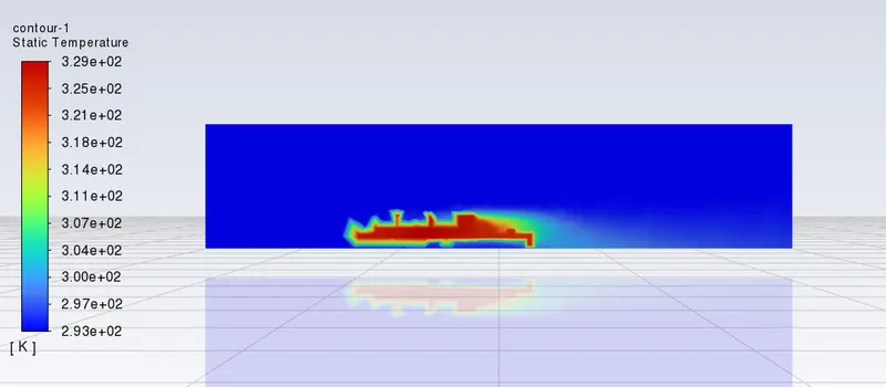
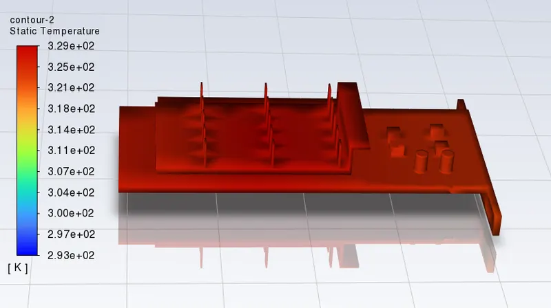
Maximum temperature of the processor
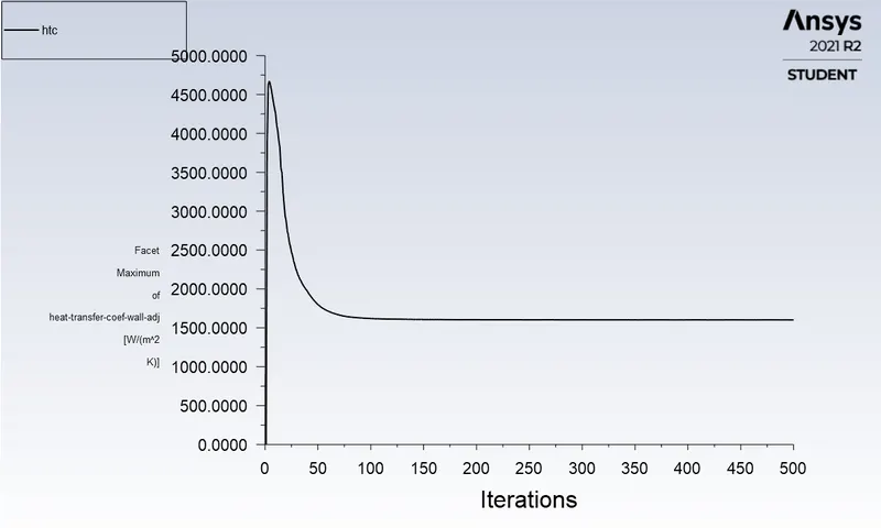
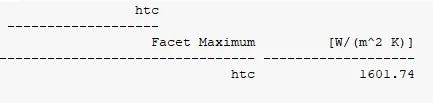
Maximum surface heat transfer coefficient of the processor
The contour temperature of the graphic card
CASE1:-
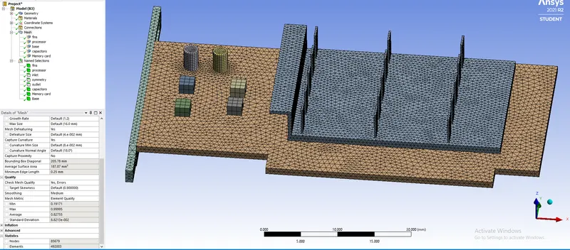
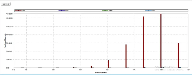
Refine mesh with body sizing and the inlet velocity 3 m/s
body sizing
processor = 0.7mm
fins = 0.5 mm
base = 0.7 mm
capacitors and memory cards = 1 mm
Encloser = 0.8 mm


Results:-
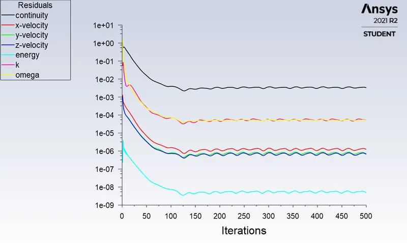
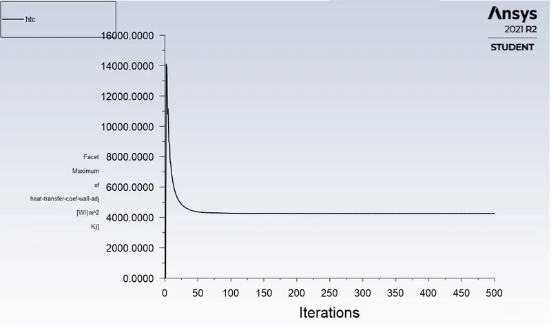
Simulation is converged as we can see the residuals are gain the steady after the 150th iteration
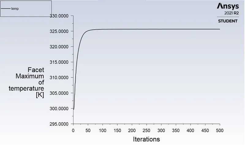
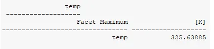
Maximum temperature of the processor
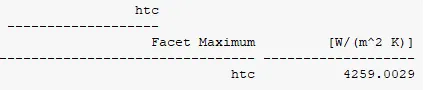
Maximum surface heat transfer coefficient of the processor
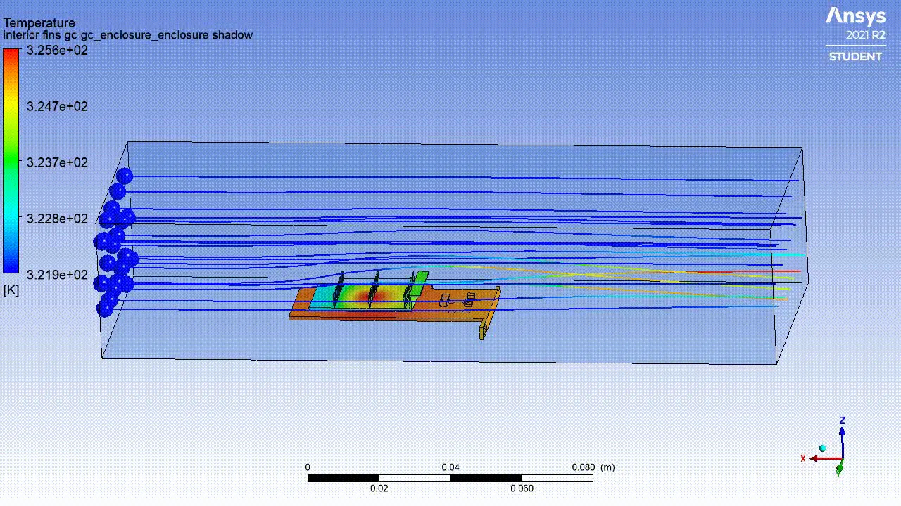
The contour temperature of the graphic card
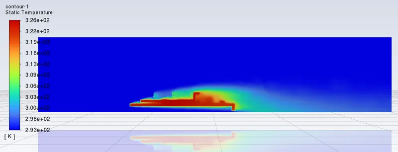
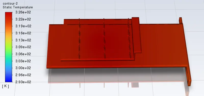
Which we can see the convection between graphic card and air
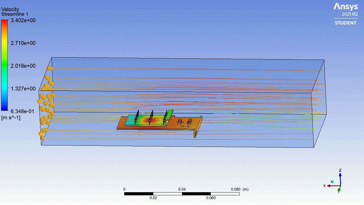
The velocity of air around the graphic card
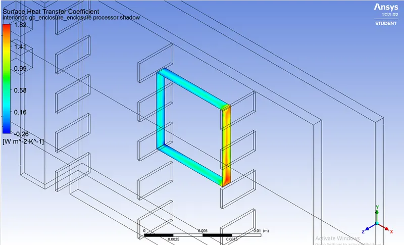
Surface heat transfer coefficient
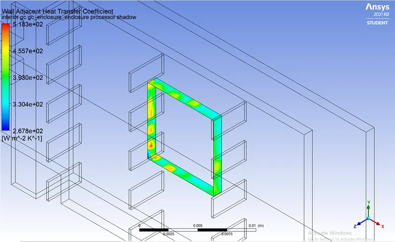
wall heat transfer coefficient
CASE2:-
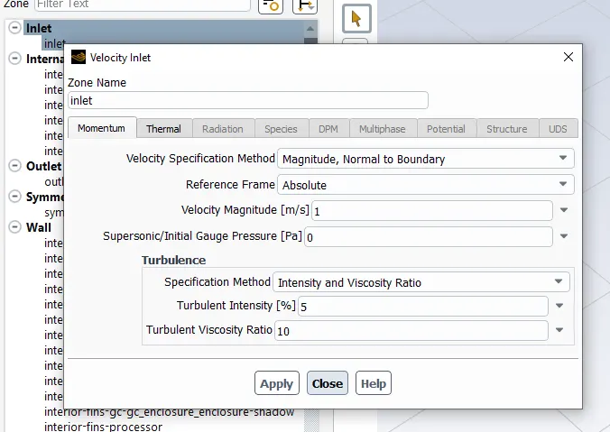
Same mesh with Inlet velocity 1 m/s
Results:-
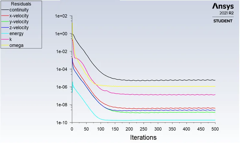
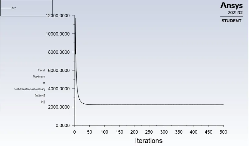
Simulation is converged as we can see the residuals are gain the steady after the 150th iteration
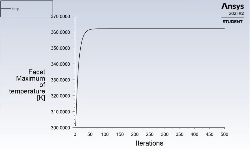
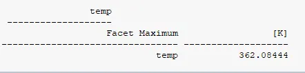
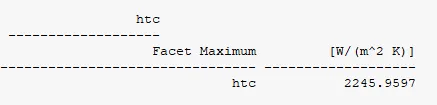
Maximum temperature of the processor
Maximum surface heat transfer coefficient of the processor
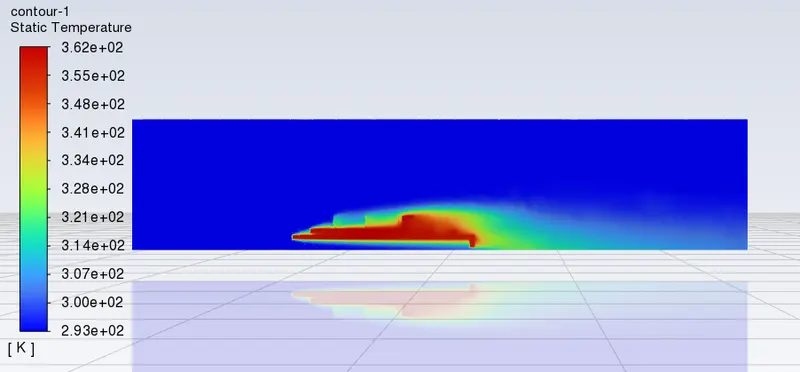
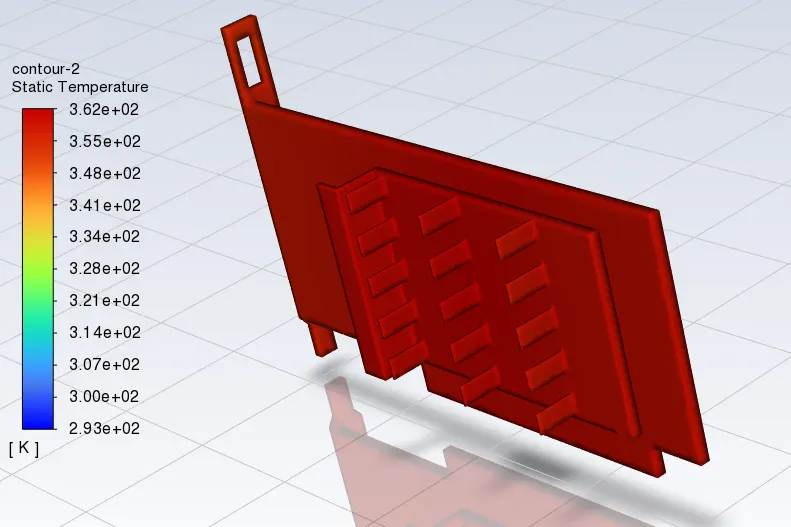
The contour temperature of the graphic card
convection between graphic card and air
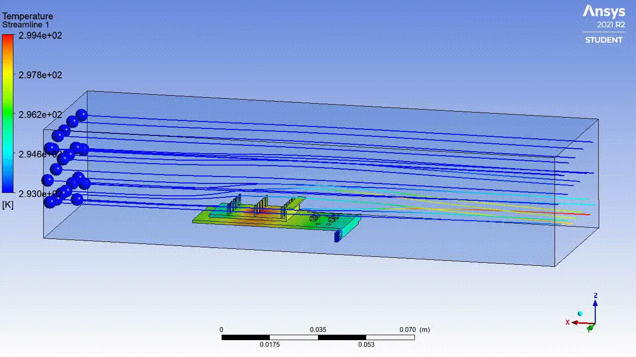
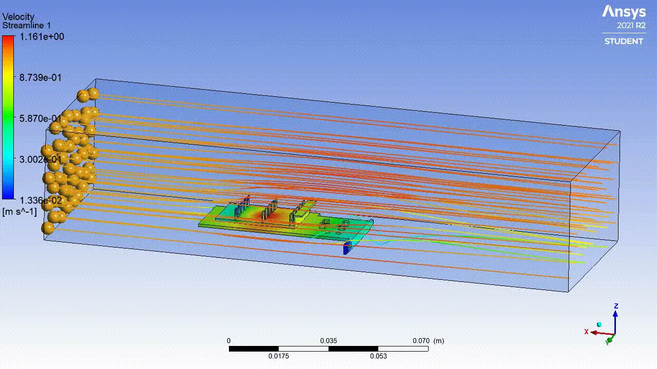
The velocity of the fluid(air) around the graphic card
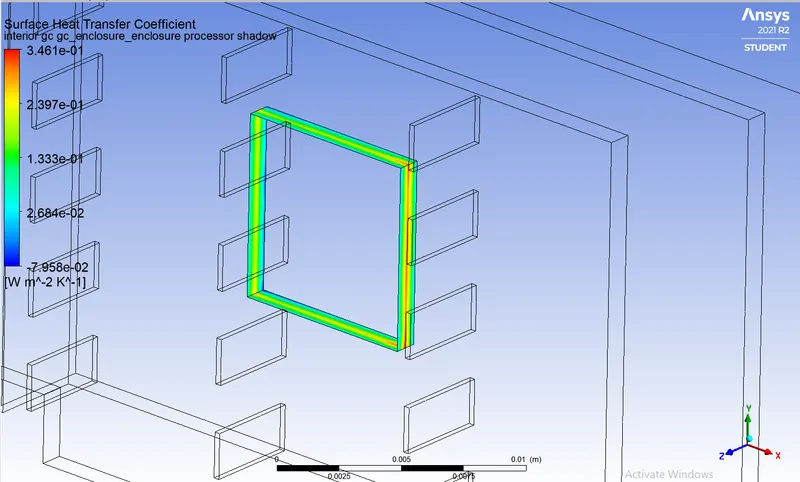
Surface heat transfer coefficient
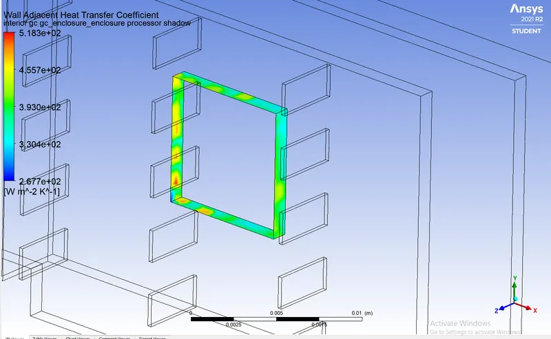
wall heat transfer coefficient
CASE3:-
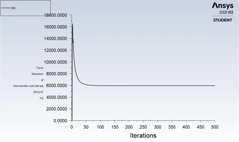
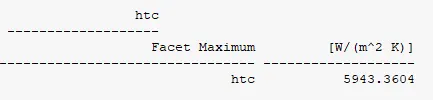
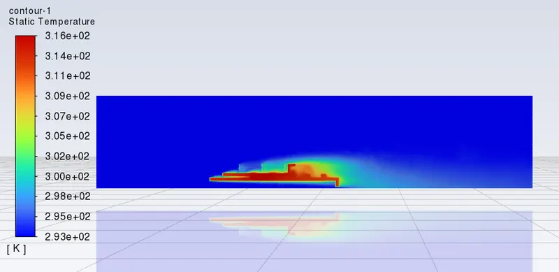
Same mesh with Inlet velocity 5 m/s
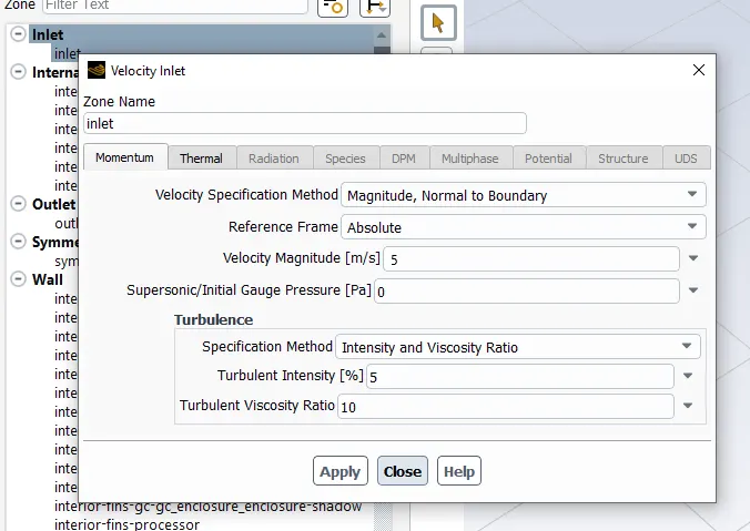
Results:-
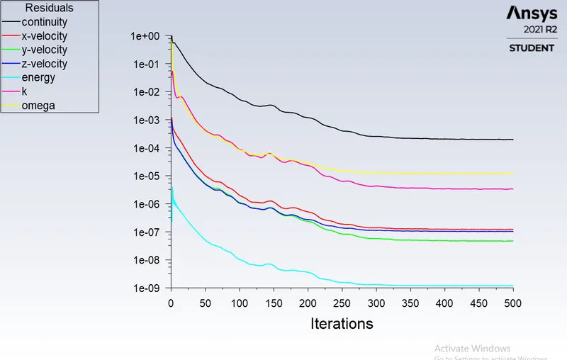
Simulation is converged as we can see the residuals are gain the steady after the 300th iteration
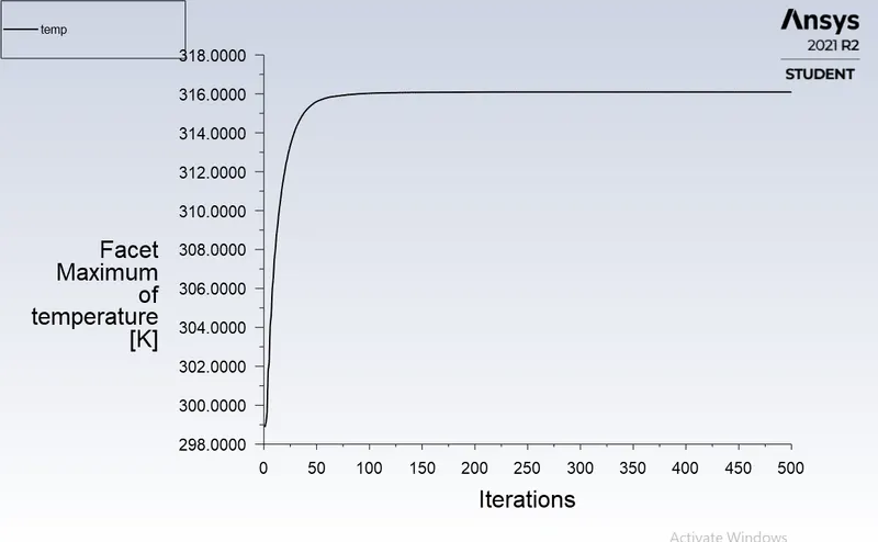
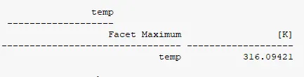
Maximum temperature of the processor
Maximum surface heat transfer coefficient of the processor
The contour temperature of the graphic card
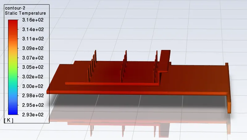
convection between graphic card and air
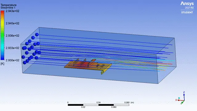
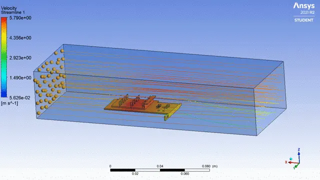
The velocity of air around the graphic card
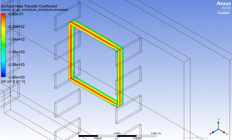
Surface heat transfer coefficient
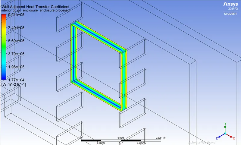
wall heat transfer coefficient
Observation:-
After the simulation
| Velocity m/s | Max temperature of the processor [K] | Max HTC of the processor `W/(m^2.k)` | |
| Baseline mesh | 3 | 328.43 | 1601.74 |
| Refine mesh | 1 | 362.08 | 2245.95 |
| Refine mesh | 3 | 325.63 | 4259.00 |
| Refine mesh | 5 | 316.09 | 5943.36 |
Comparing the above CASES
In course mesh and refine mesh of velocity 3 m/s we can see the slight temperature difference and the wall HTC as a large difference between these simulations so that finer mesh will give the accurate value
And also we can see increasing in HTC and a decrease in temperature with respect to velocity increase
Potential hotspots on the model
Validation:-
Forced convection on flat plate
Flat plate in laminar flow
The local Nusselt number for laminar flow over a flat plate, at a distance downstream from the edge of the plate, is given by

The average Nusselt number for laminar flow over a flat plate, from the edge of the plate to a downstream distance , is given by

Reynolds number (Re)
`R_e = (rho*U*L)/(mu)`
`R_e =2738.34`
Prandtl number (pr)
`Pr = (c_p.mu)/(k)`
`Pr=0.707`
Nusselt number(Nu)

where
h is the convective heat transfer coefficient of the flow,
L is the characteristic length,
k is the thermal conductivity of the fluid.
so we can write
`(hL)/k=0.332*Re_x^(1/2)*Pr^(1/3)`
`h=(0.332*Re_x^(1/2)*Pr^(1/3)*k)/L`
`h=(0.332*2738.34^(1/2)*0.707^(1/3)*0.020)/0.008`
`h =38.69`W/(m^2 K)
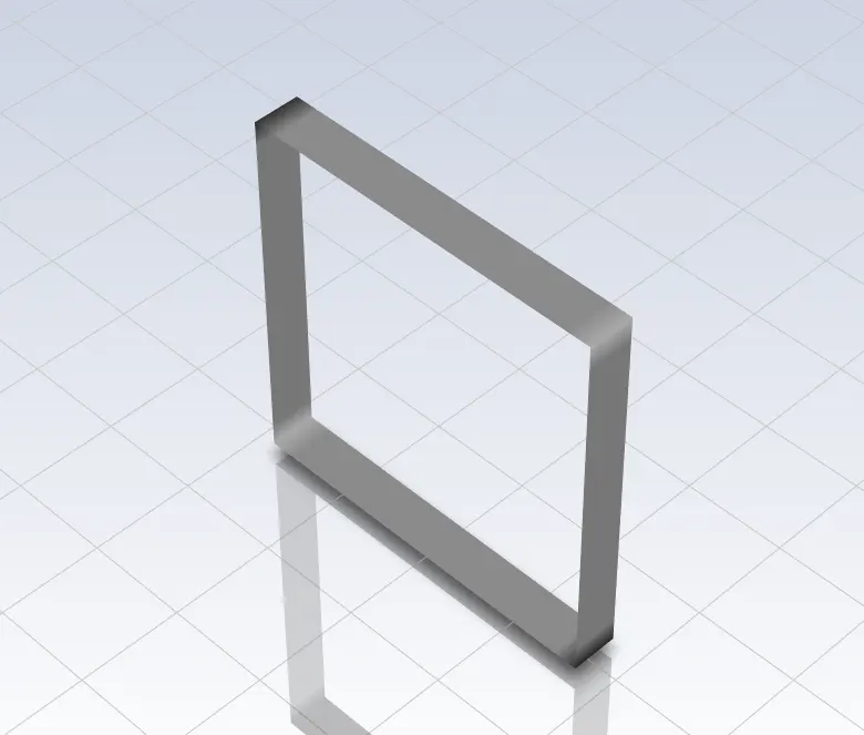
But HTC of the encloser-processor shadow as shown below is 14.79 W/(m^2 K)
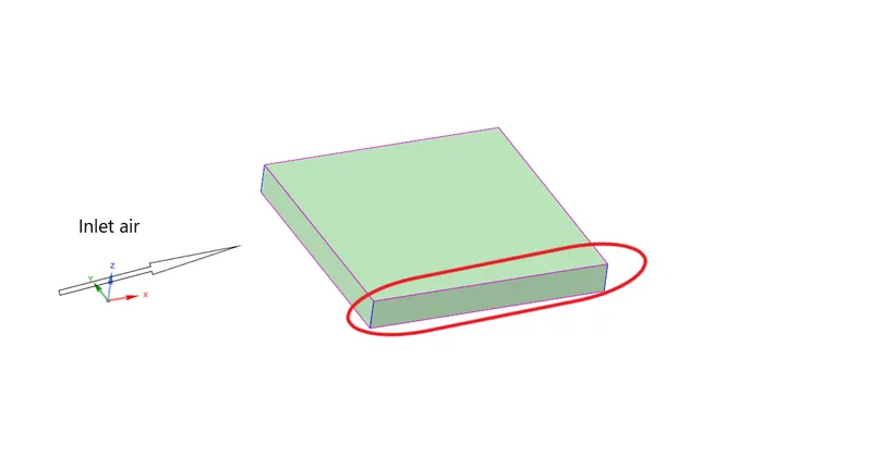
The above calculation is for one side of the processor as shown below
Conclusion:-
- course mesh and refine mesh of velocity 3 m/s we can see the slight temperature difference and the wall HTC as a large difference between these simulations so that finer mesh will give the accurate value
- And also we can see increasing in HTC and a decrease in temperature with respect to velocity increase
- As velocity of incoming air increased, the maximum temperature reached was decreased. This is due to the fact that, as air velocity increases, heat transfer convective coefficient increases so heat transfer to the surrounding increases and temperature attained by the material decreases.
- As per the direction of air velocity, heat transfer for fins changes from left to right as shown in the temperature contour on Fin-base section.