Week 6 - CHT Analysis on a Graphics card
AIM: To perform a steady-state conjugate heat transfer analysis on a model of a Graphics Card.
OBJECTIVES:
- Run the simulation by varying the velocity from 1 m/sec to 5 m/sec for at least 3 velocities and discuss the results.
- Find out the maximum temperature and heat transfer coefficient by the processor.
- Prove that the simulation has achieved convergence with appropriate images and plots.
- Identify potential hotspots on the model.
THEORY:
Conjugate Heat Transfer
The key element in having a conjugate heat transfer, as the name suggests the thermal interaction between a fluid and a solid region. This is the basic and most important element of a conjugate heat transfer simulation. If we want to divide it, Into solid regions we are simulating the heat conduction, heat conduction is basically the diffusion of heat due to direct contact. In the fluid regions, we are dealing with Convection of heat, this is the kind of transfer of thermal energy due to the movement of fluid elements. At the interfaces between these two regions, we have the thermal coupling that's why the name is Conjugate heat transfer because we are considering the transfer of mass and thermal energy at the same time both in solid and fluid.
Advantages:
Conjugate Heat Transfer has many advantages that's why it is used.
- Accurate and fast
- Suited for complex scenarios
- Assemblies: no limits on the number of regions
- All types of region combinations like solid-fluid, fluid-fluid can be simulated.
Applications of CHT:
- Cooling of electronic devices
- Heat exchangers
- HVAC
- Heating
- Ventilating
- Air conditioning
- Combustors and Burners
- Gas turbine design
- Engine cooling
- Home appliances
- ...
CONJUGATE HEAT TRANSFER ANALYSIS ON A GRAPHICS CARD:
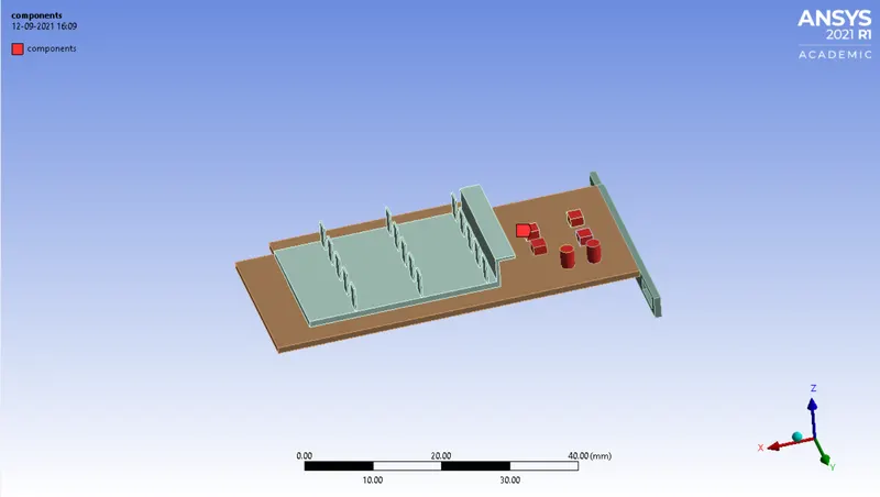
We will be using the made-up geometry but it contains the features that the actual Graphics card would have. The Graphics card is a three-dimensional model containing a base, processor, fins, and six components. In the graphics card, the processor is the main heating part of the assembly. In the graphics card model, the processor is directly mounted over the base, on the processor, there is a heat sink provided which will have more surface area to dissipate the heat. The heat generated from the processor is conducted through the heat sink. Hence heat sink is provided to reduce the overheating of the processor. The fins are placed to provide efficient cooling for the processor using air as a fluid. The fins of the heat sink increase the effective area of convective heat transfer. Forced convection occurs from the fins to the fluid. The fins act as a heat exchanger, it basically takes the heat from the sources i.e. processor, and releases it to the air through convection.
A graphics card is kept inside an enclosure with moving air. Our objective is to determine the Heat transfer coefficient with respect to different magnitudes of velocity.
The steps used for solving the problem:
Geometry:
1. Loaded the Graphics card model into the SpaceClaim.
2. Enabled share topology of the main component so that the mesh and physics information or necessary information can be shared between different zones and conformal mesh can be achieved.
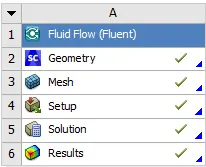
3. To achieve conjugate heat transfer between the fluid and the solid wall we had to choose the share option under the workbench tool this is very important if it is not done we will not see the interfaces where information is being shared so this is very important if we don't do this step and directly go to the meshing interface the mesh will definitely fail. Basically, this particular step takes care of creating the interfaces so that we have one interface.
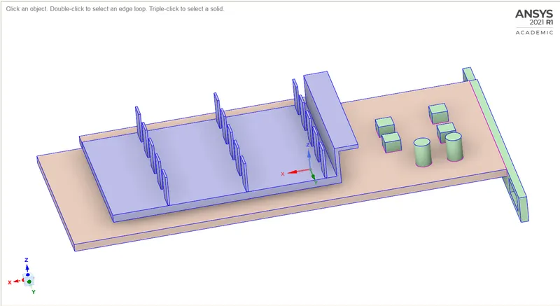
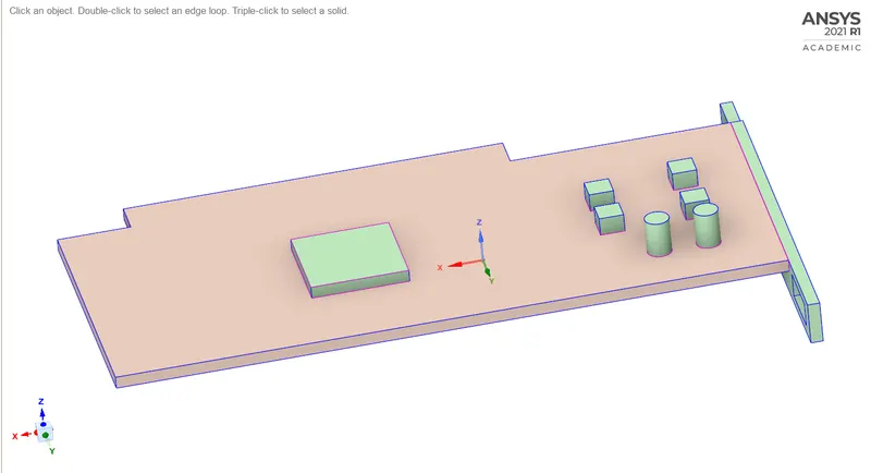
We can see these pink circles that basically tell us where information is being shared.
Mesh:
1. After the geometry setup opened the Mesh.
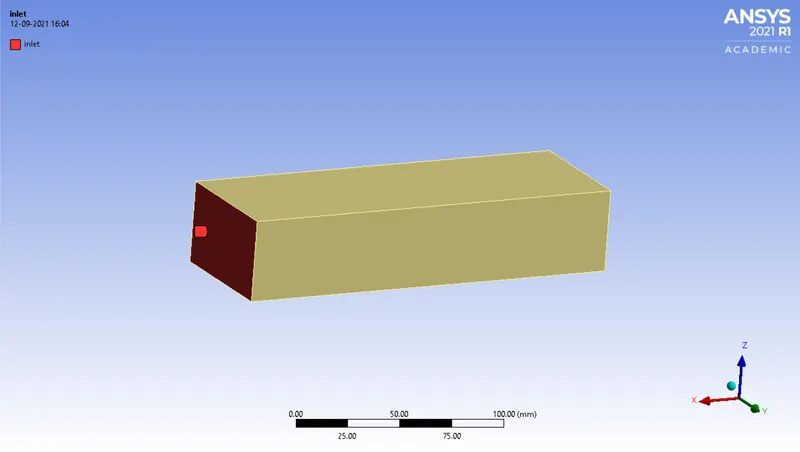
2. Selected the faces and named them.
Inlet
Outlet
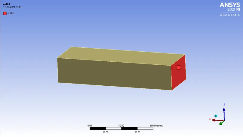
Symmetry
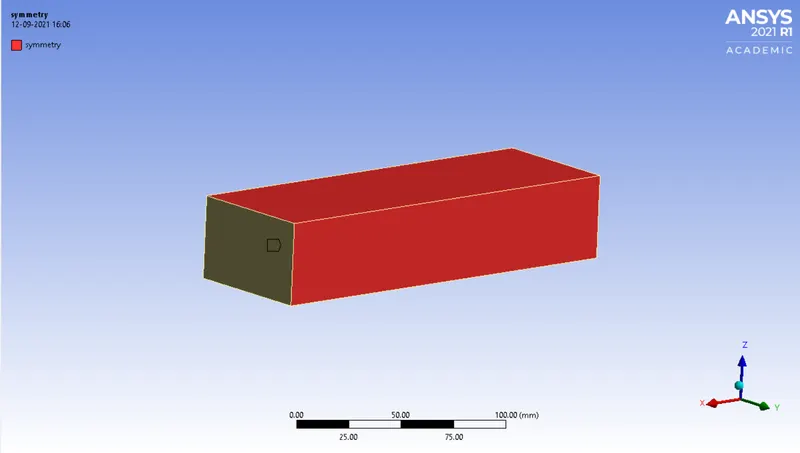
Processor
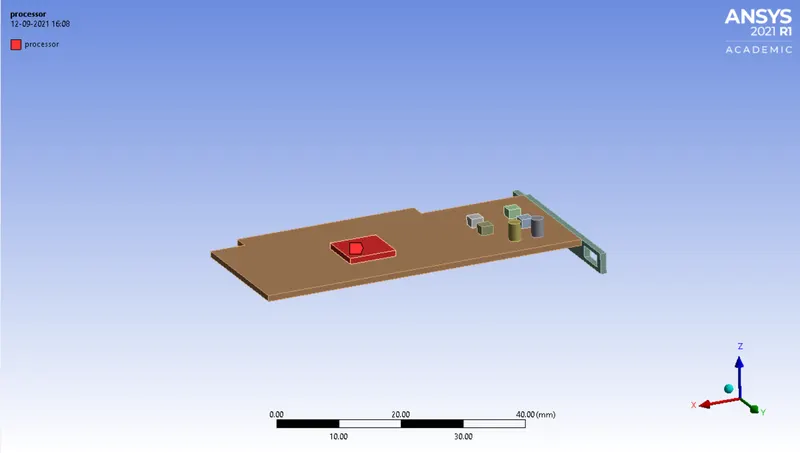
Fins
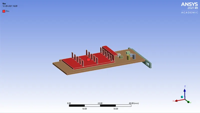
Components
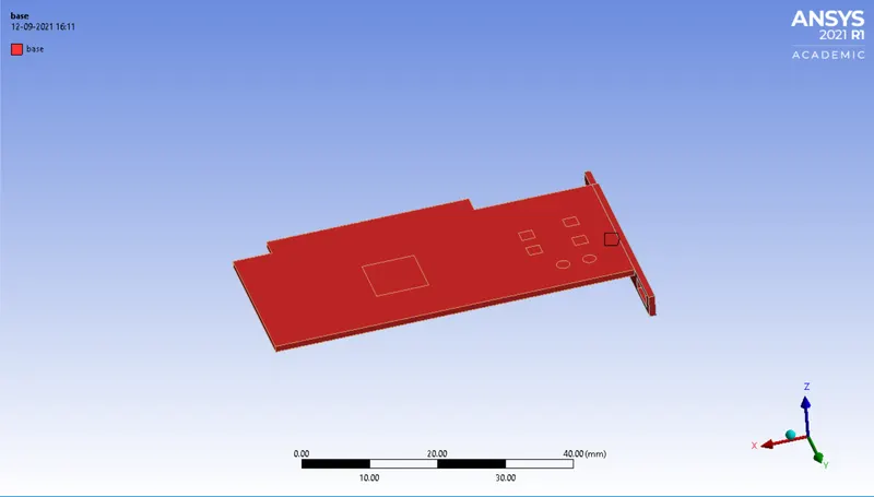
Base
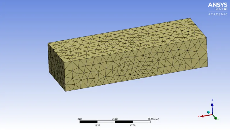
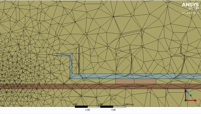
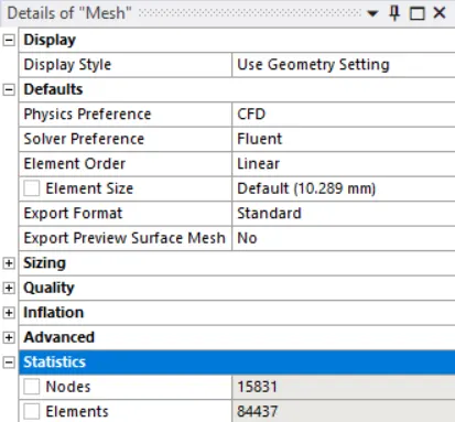
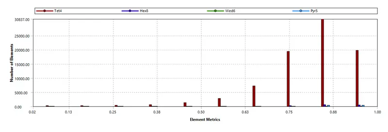
Baseline Mesh:
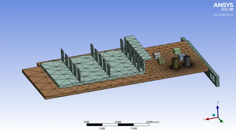
Section plane
Setup:
1. After meshing, opened the fluent Setup, In the general setting selected a pressure-based solver, steady-state time simulation, absolute velocity formulation, and enabled energy option.
2. K-omega SST turbulence model is selected.
3. The solid zones and fluid zones are defined in the cell zones under the Physics tab.
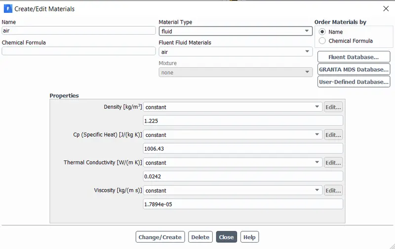
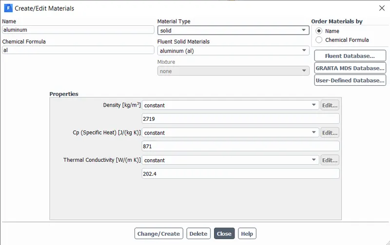
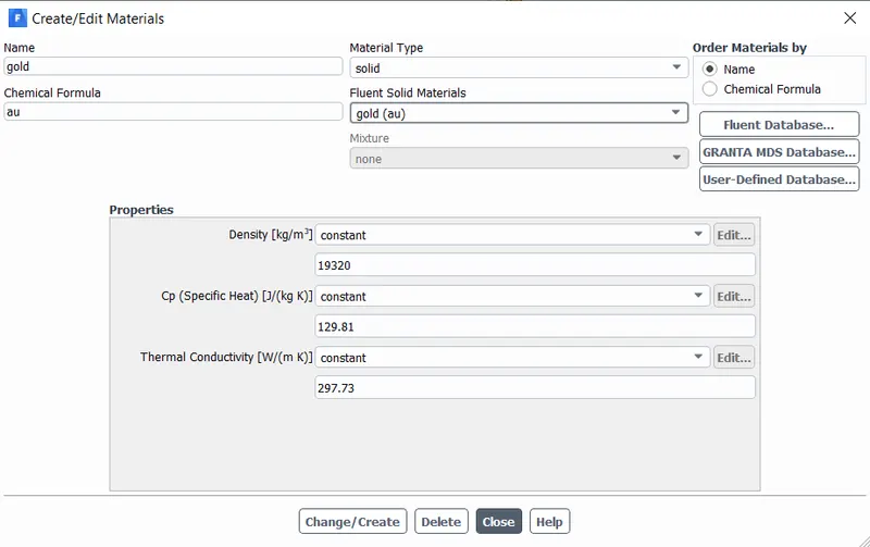
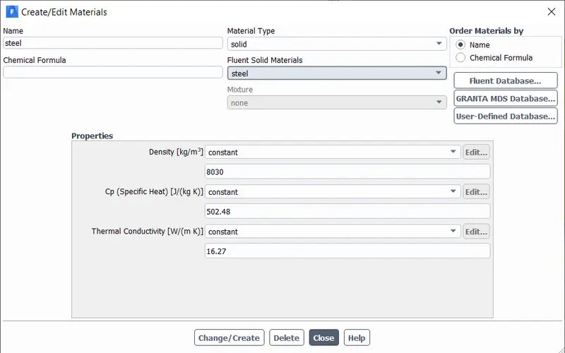
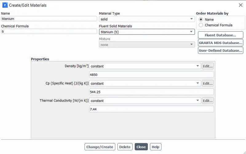
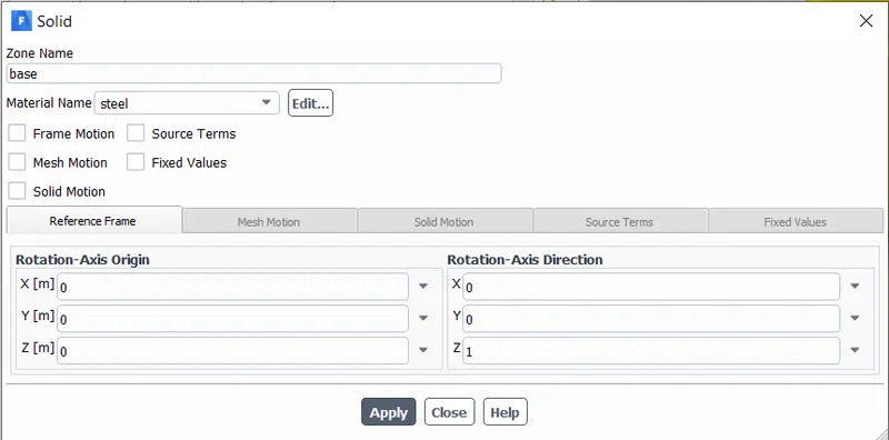
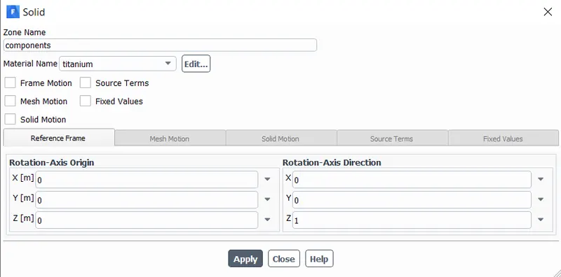
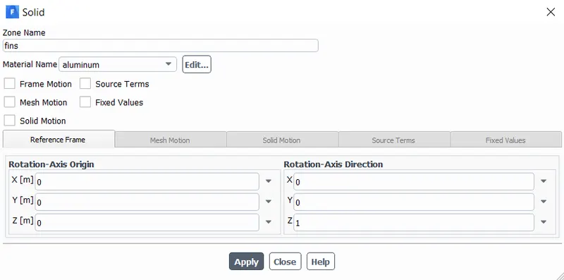
4. Materials are chosen in the Create/Edit Material. The materials are then specified for the different components of the graphics card. The material's properties are constant and do not change under any condition.
Materials:
Different materials were assigned for different components,
Steel for base:
titanium for components:
Aluminum for fins:
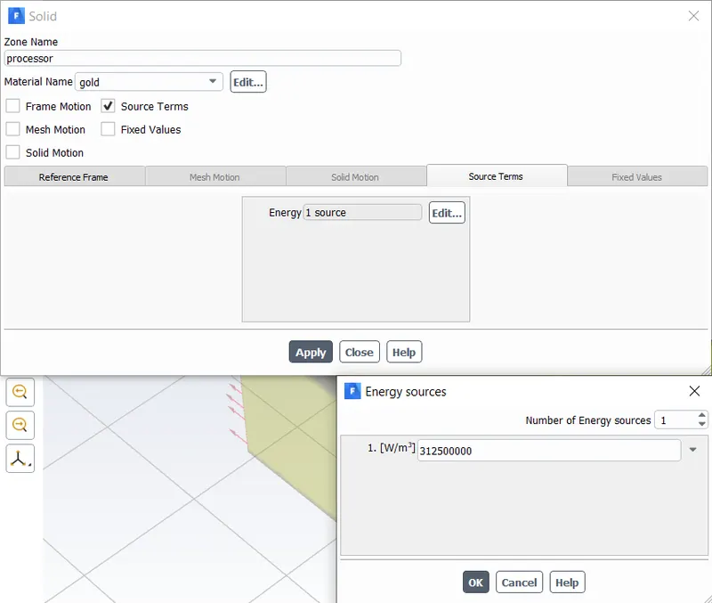
Gold for processor:
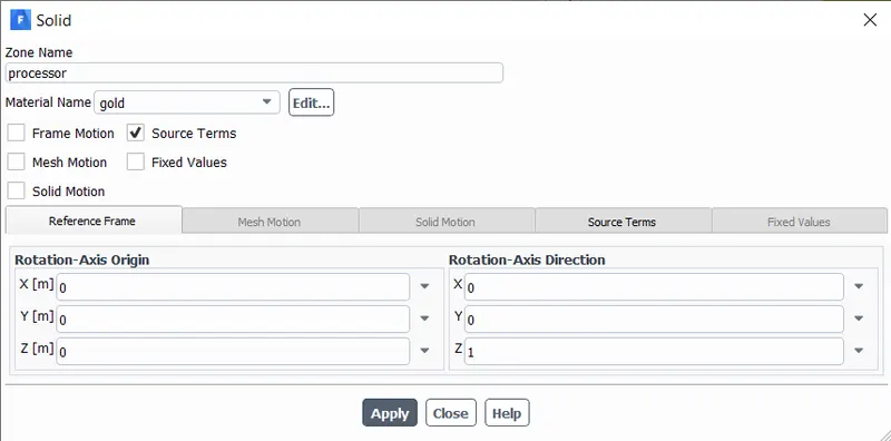
Heat Source calculation:
Processor Power = 20 watts
Length of the processor (L) = 8 mm
The breadth of the processor (b) = 8 mm
The thickness of the processor (h) = 1 mm
The volume of the processor (L*b*h) = `64 mm^3`
=`0.000000064 m^3`
The heat generated by processor = Processor power/Volume of the processor
= 20/0.000000064
= 312500000 `W /m^3`
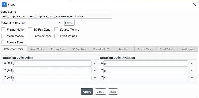
Air as the fluid:
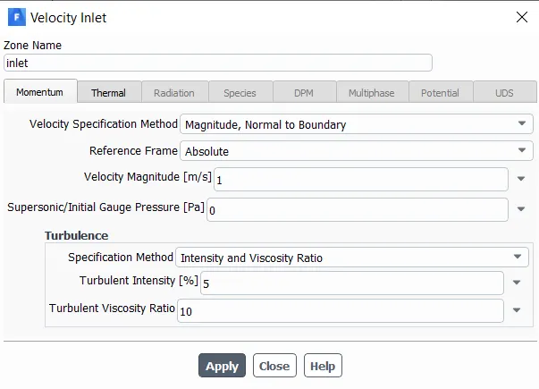
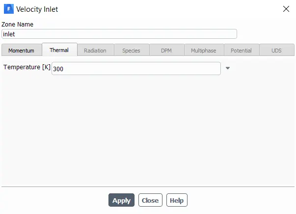
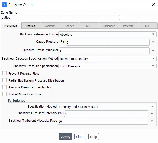
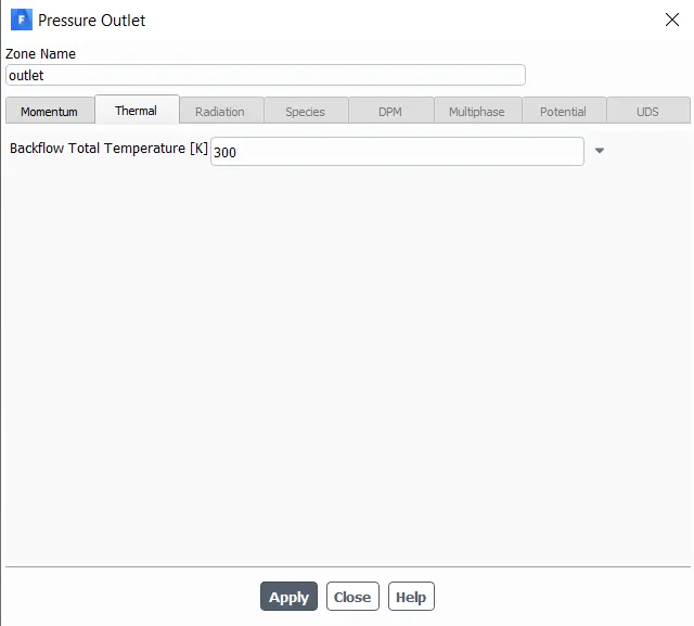
Boundary condition:
Solution:
Initialization --> select method = Hybrid --> click t=0 Initialize
Run calculation --> No. of iterations = 500 and pressed calculate.
Results:
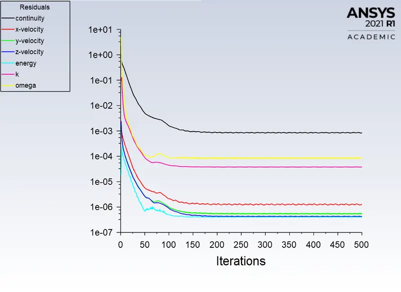
Residual plot: From the residual plot as shown below, the solution can be considered as converged as the variation of residuals is less and follows the same pattern. It can be said that the solution is converged around 150 iterations.
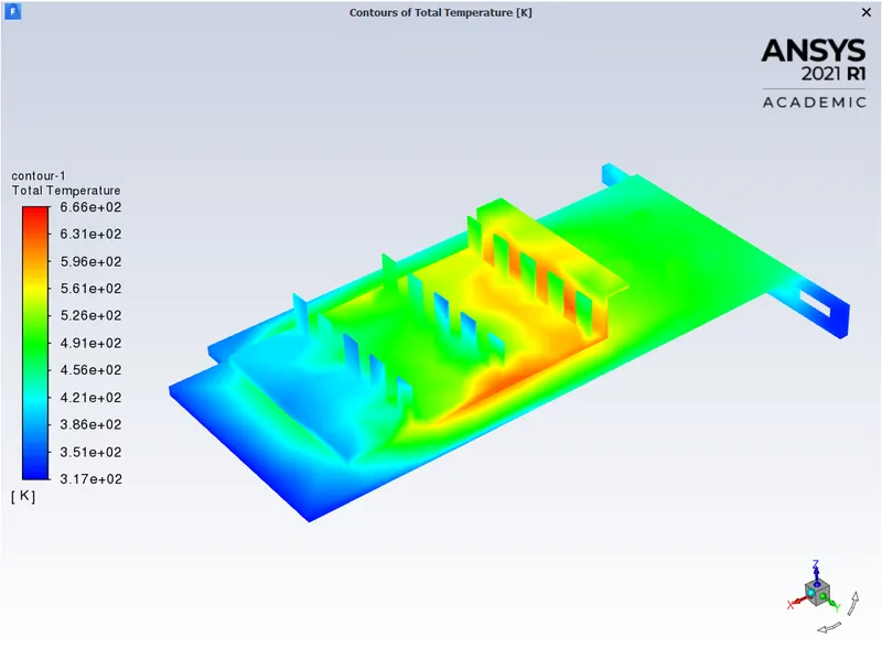
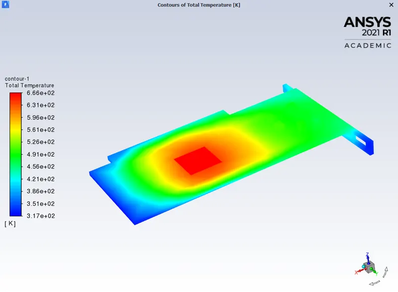
Total temperature:
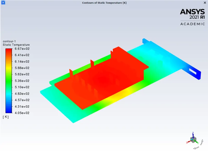
Static temperature:
The total temperature at base:
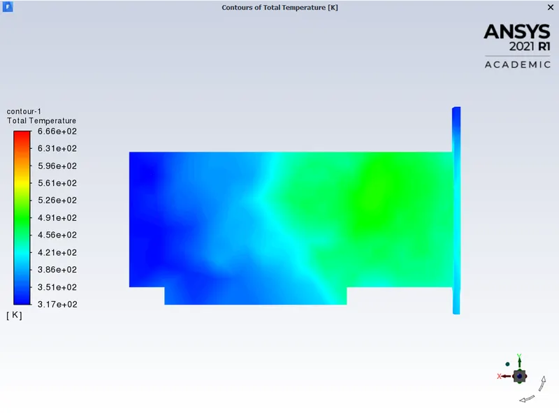
The total temperature at the bottom face of the base:
Potential hotspot at base:
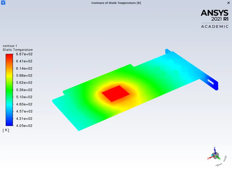
Potential hotspot at the bottom face of the base:
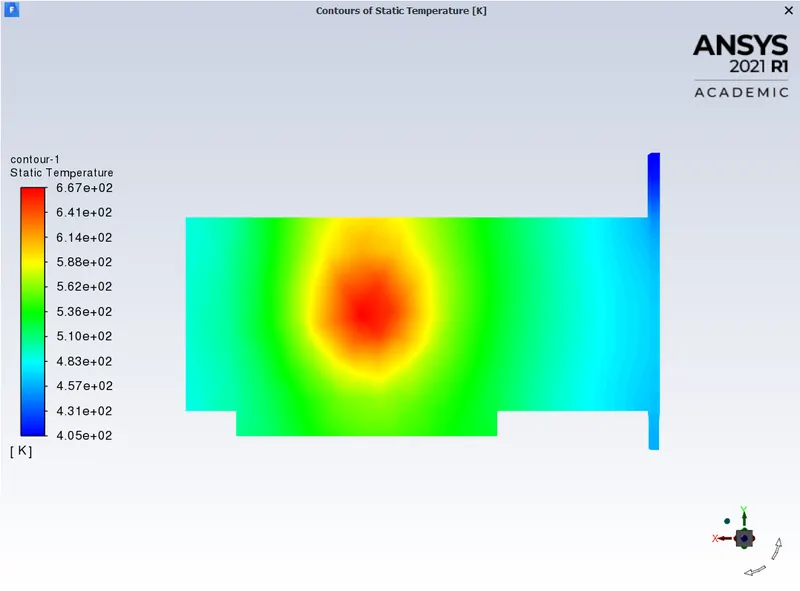
The total temperature at fins:
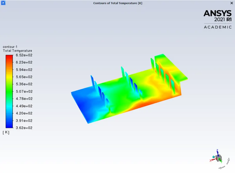
The total temperature at the bottom face of the fins:
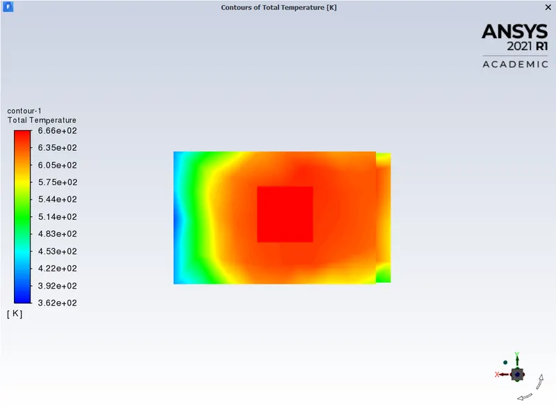
Potential hotspot at fins:
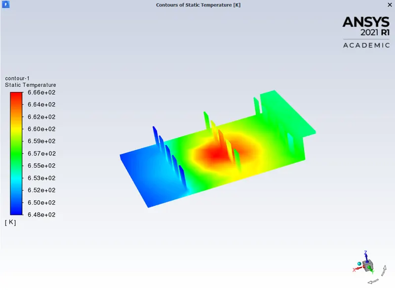
Potential hotspot at the bottom face of the fins:
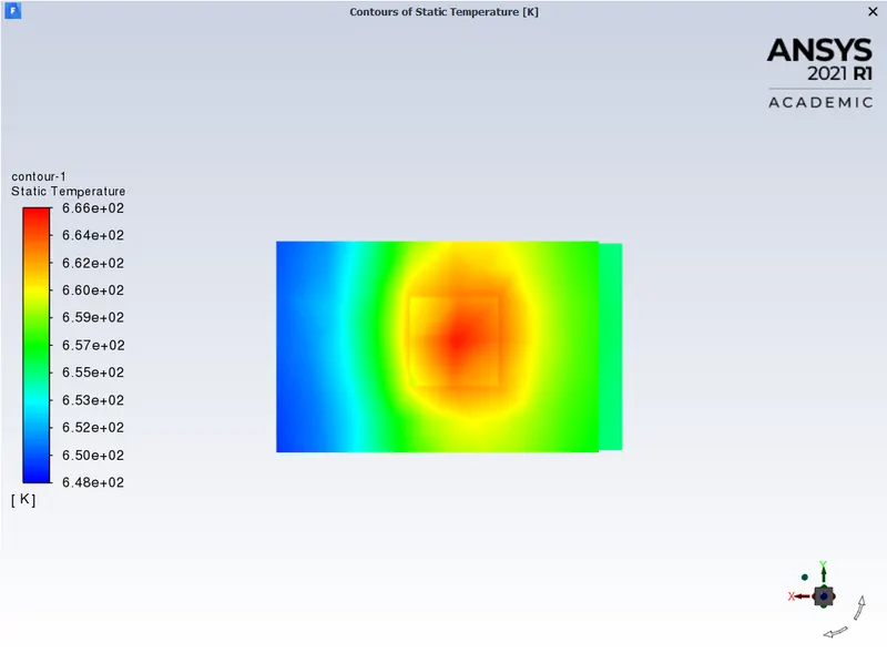
The temperature at the processor:
The maximum value of temperature at the processor is 665.8619 k.
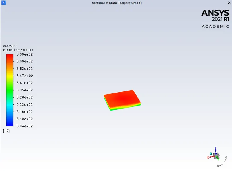
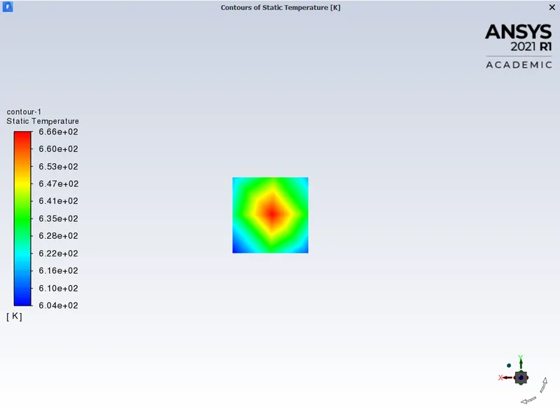
The temperature at the bottom face of the processor:
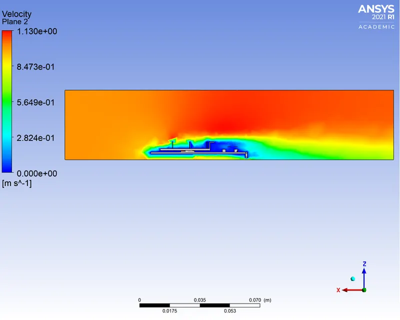
Velocity contour at XZ plane where y=0:
Temperature contour at XZ plane where y=0:
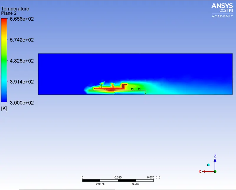
Wall HTC at graphics card:
The maximum value of the Wall heat transfer coefficient is `995.5381 W/(m^2K)`
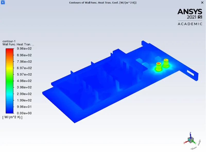
Wall HTC at fins:
The maximum value of the Wall heat transfer coefficient at fins is `152.5389 W/(m^2K)`
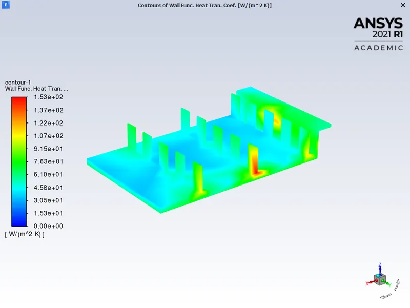
Wall HTC at processor:
The maximum value of the Wall heat transfer coefficient at the processor is `78.13793 W/(m^2K)`
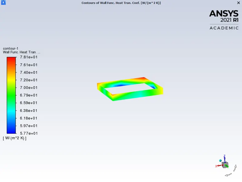
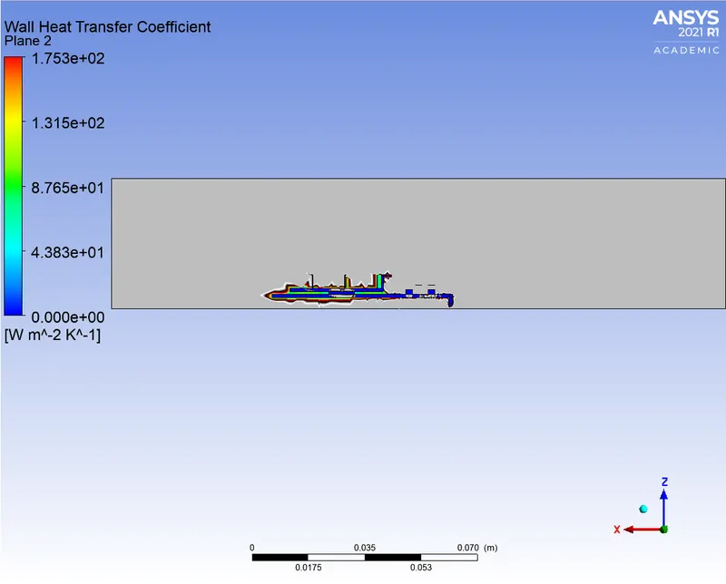
Wall HTC at XZ plane where y=0:
The maximum value of the Wall heat transfer coefficient is `175.307 W/(m^2K)`
Refined Mesh:
Results are coarser in baseline mesh, for getting fine results we had to refine the mesh. In this case, we are using a finer mesh up to the allowed limit.
For structural and fatigue analysis quad and hex elements are preferred, for the crash and non-linear analysis we still try to get as many quad elements as possible. For casting simulation, triangular elements are preferred over quads, The reason for doing this is generally for balance between results accuracy and simulation time.
When any geometry resembles both normal shape and complex shape, the Ansys workbench mesh algorithm meshes normal shape geometry into hexahedral mesh whereas complex geometry in the tetrahedral mesh. In our case, we have a similar type of geometry where we have a processor and capacitors as normal shape geometry and the base and fins as complex geometry.
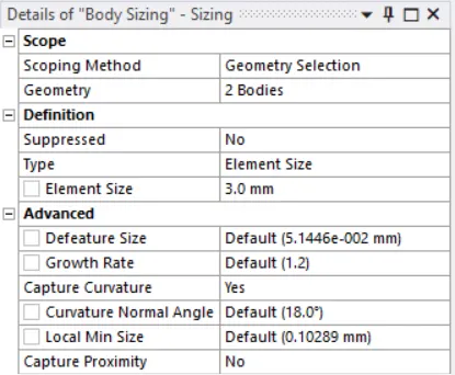
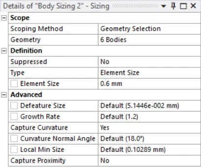
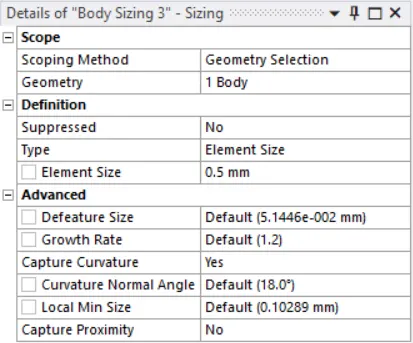
In order to get the mesh finer in the region of the graphics card following mesh settings were made.
Base:
Components:
Processor:
Fins:
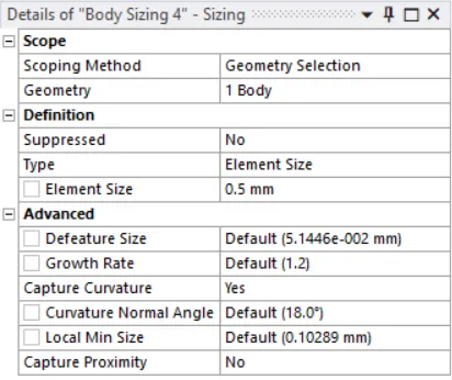
Enclosure:
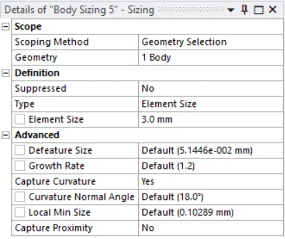
Final mesh:
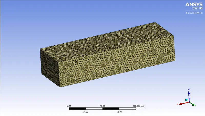
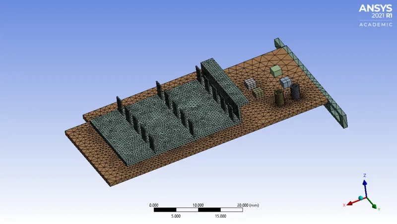
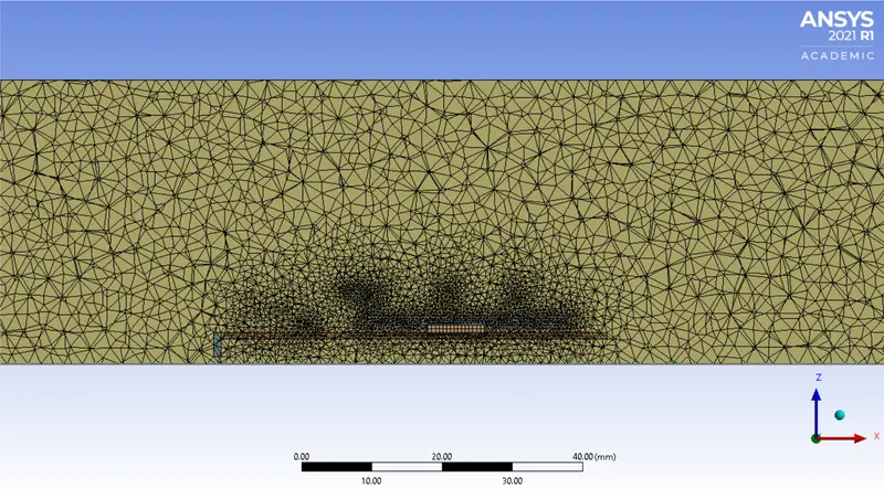
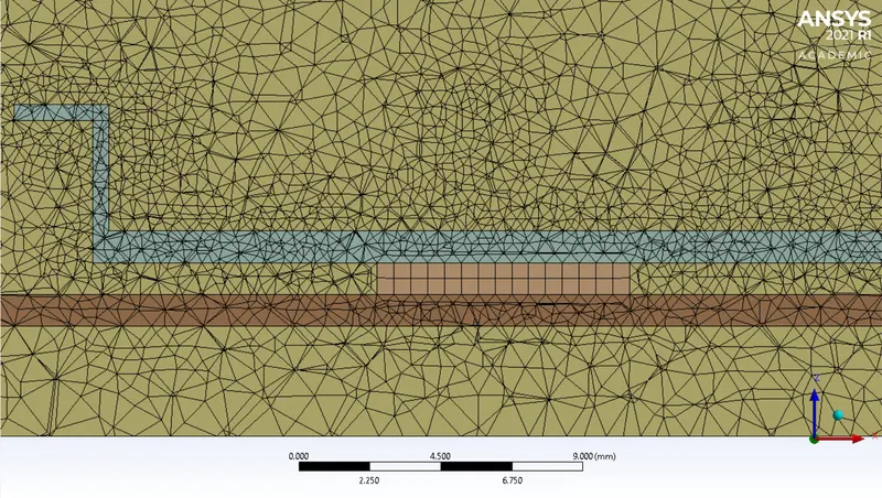

The number of elements achieved is 500706 which is less than 512000 which is a limit of the Ansys Student version.
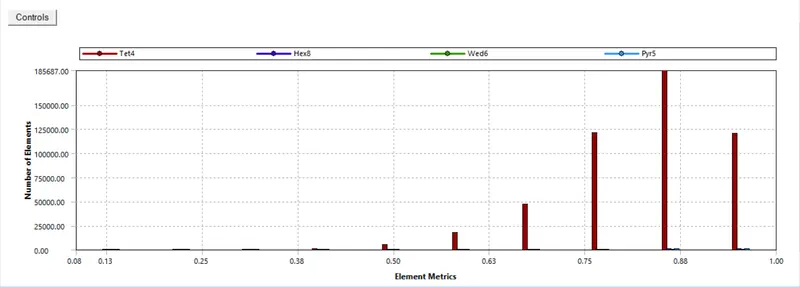
Results: We are studying the refined case for 5 different values of inlet velocity.
Case 1:
Velocity = 1 m/s
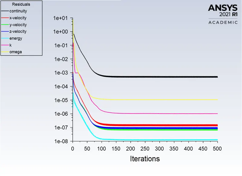
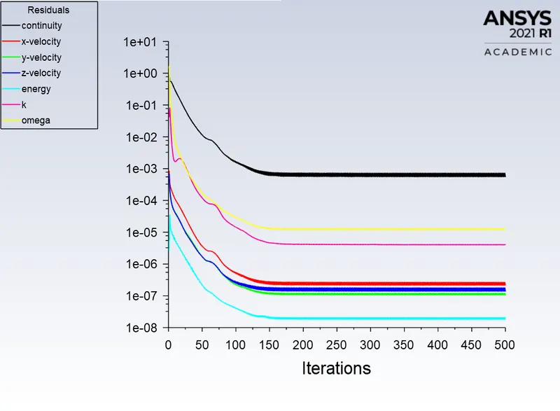
Residual plots:
From the residual plot, as shown below, the solution can be considered as converged as the variation of residuals is less and follows the same pattern. It can be said that the solution is converged around 125 iterations.
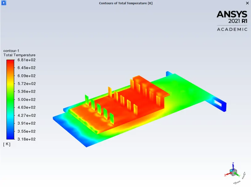
Total Temperature:
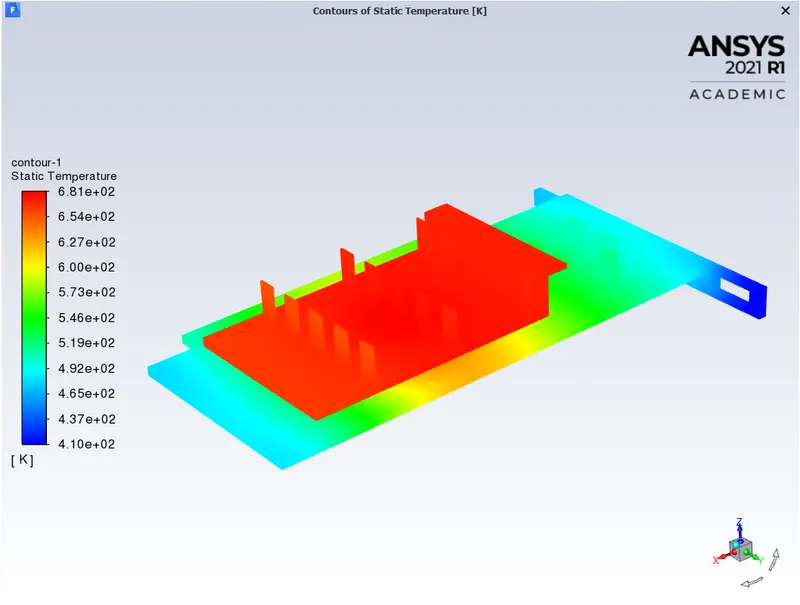
Static Temperature:
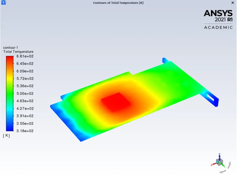
The total temperature at base:
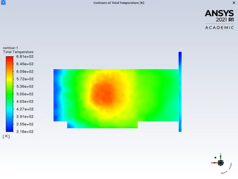
The total temperature at the bottom face of the base:
Potential hotspot at base:
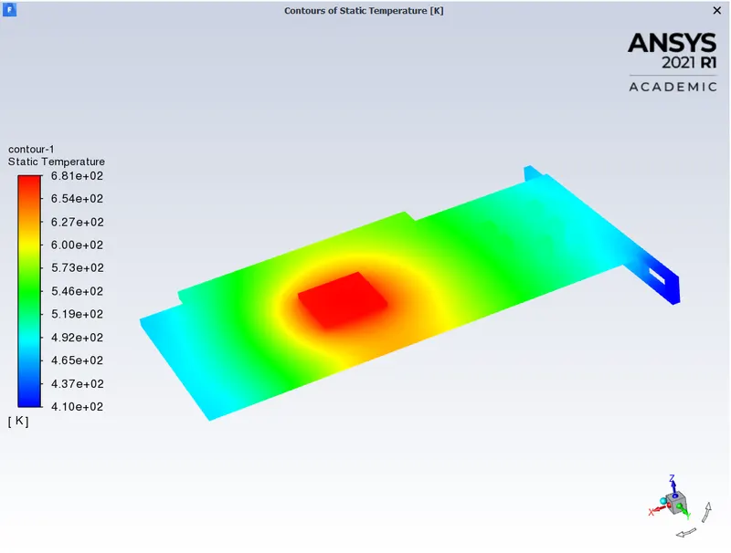
Potential hotspot at the bottom face of the base:
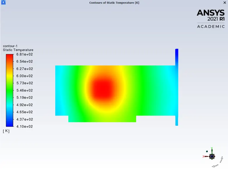
The total temperature at fins:
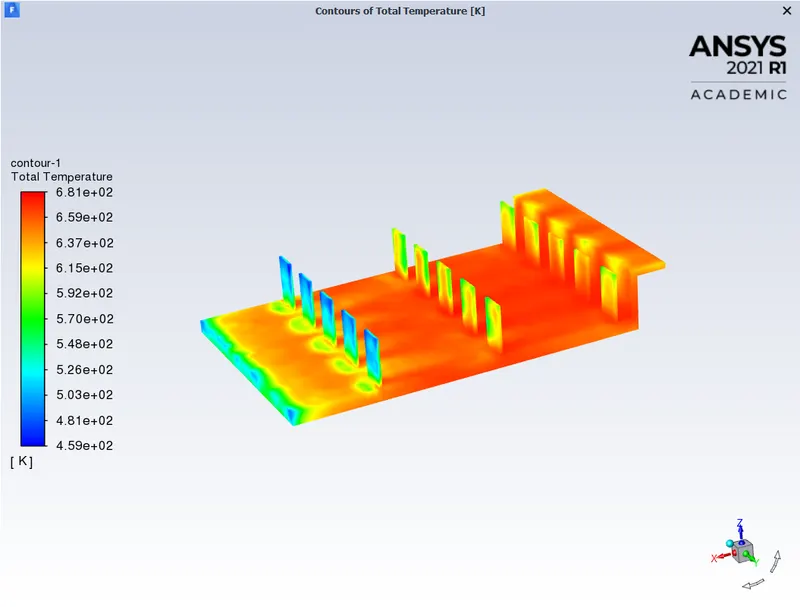
The total temperature at the bottom face of the fins:
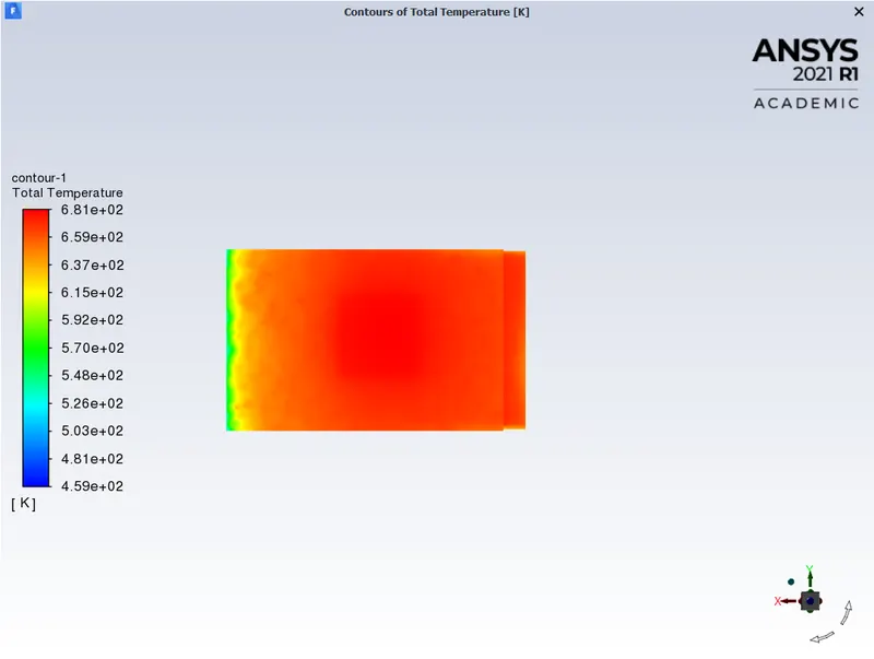
Potential hotspot at fins:
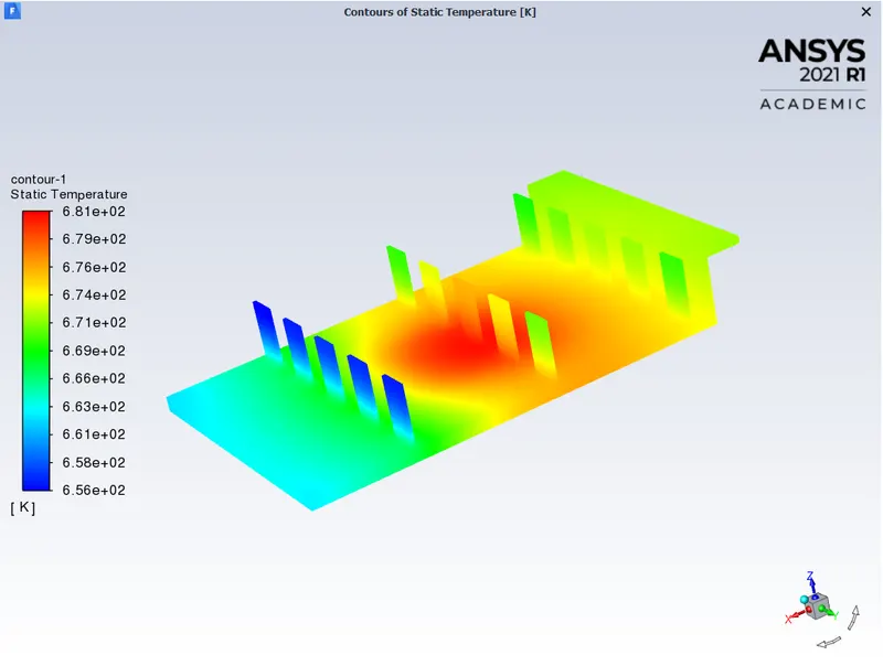
Potential hotspot at the bottom face of the fins:
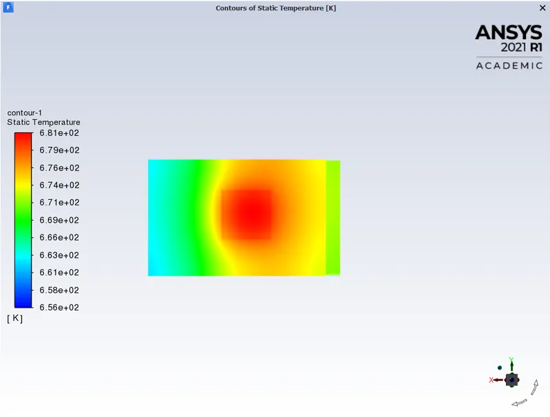
The temperature at the processor:
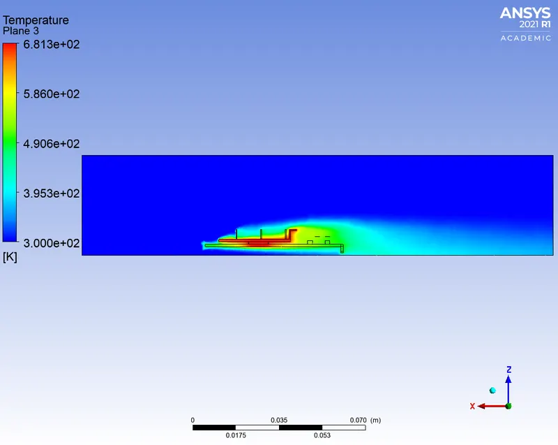
The maximum temperature at the processor is 681.3875 K
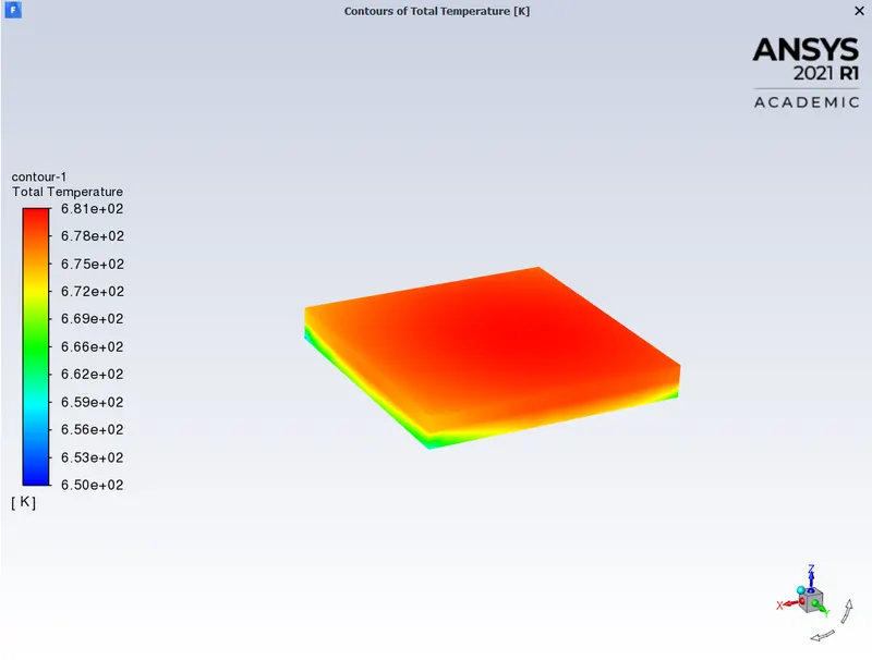
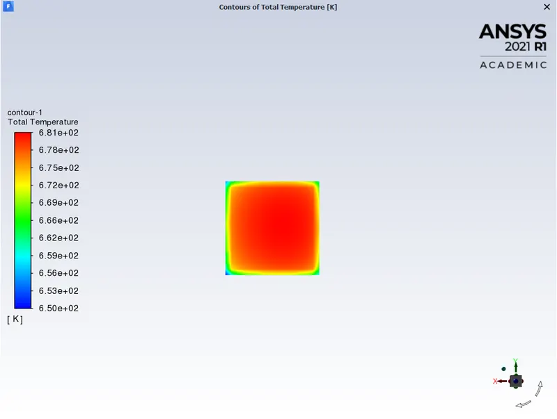
The temperature at the bottom face of the processor:
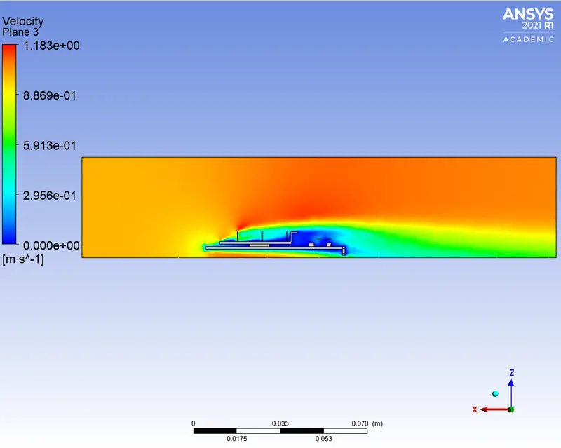
Velocity contour at XZ plane where y=0:
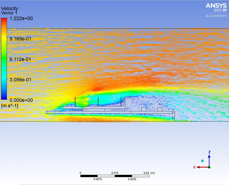
Velocity vector:
Temperature contour at XZ plane where y=0:
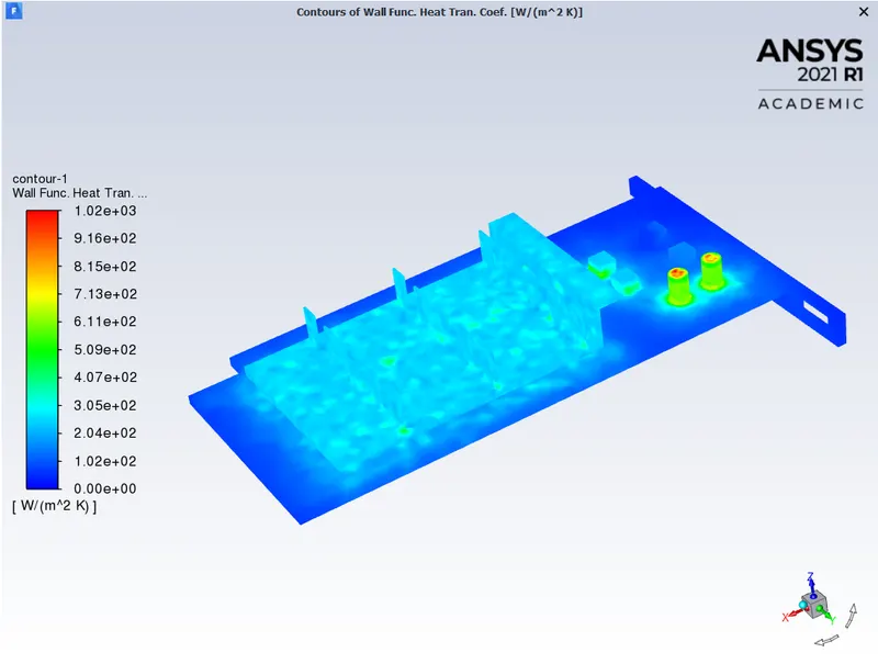
Wall HTC at graphics card:
The maximum value of the Wall heat transfer coefficient is `1018.134 W/(m^2K)`
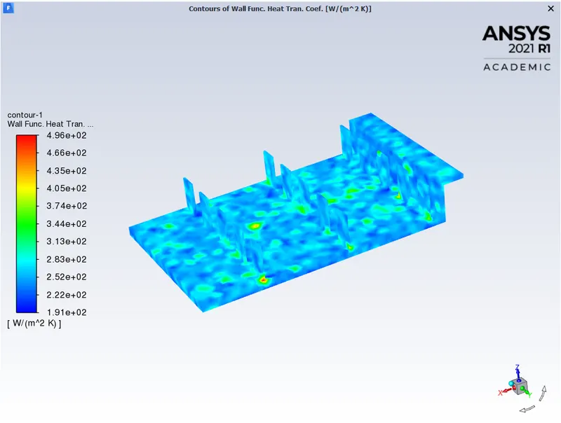
Wall HTC at fins:
The maximum value of the Wall heat transfer coefficient at fins is `496.2925 W/(m^2K)`
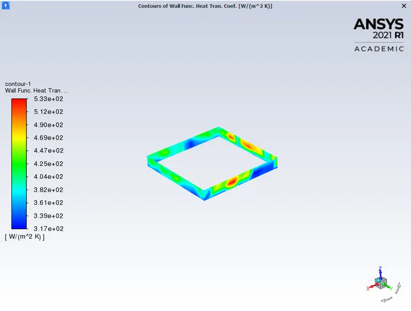
Wall HTC at processor:
The maximum value of the Wall heat transfer coefficient at the processor is `533.4125 W/(m^2K)`
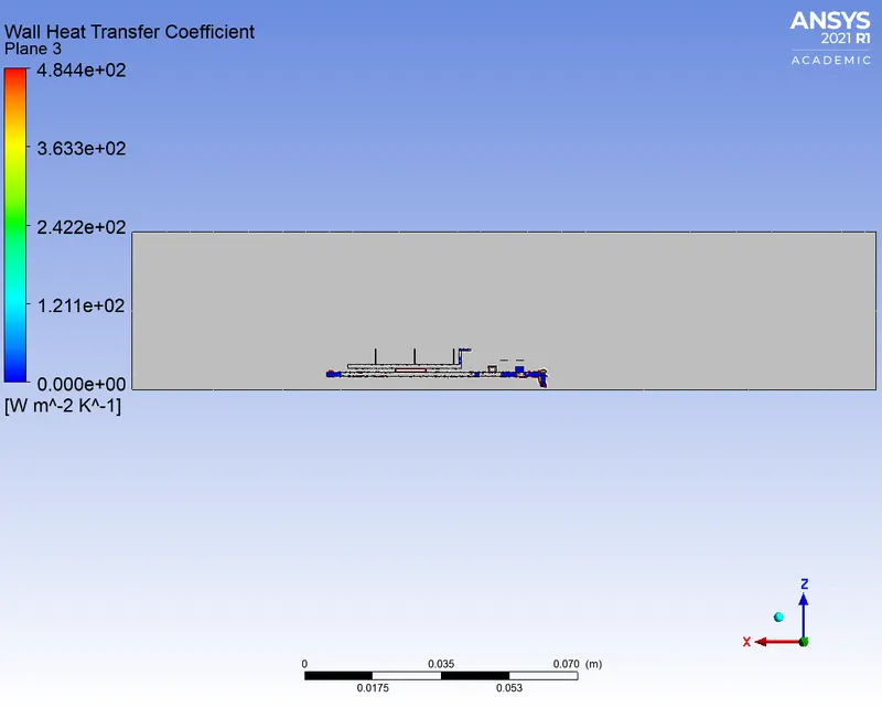
Wall HTC at XZ plane where y=0:
The maximum value of the Wall heat transfer coefficient is `484.412 W/(m^2K)`
Case 2:
Velocity = 2 m/s
Residual plot:
From the residual plot, as shown below, the solution can be considered as converged as the variation of residuals is less and follows the same pattern. It can be said that the solution is converged around 150 iterations.
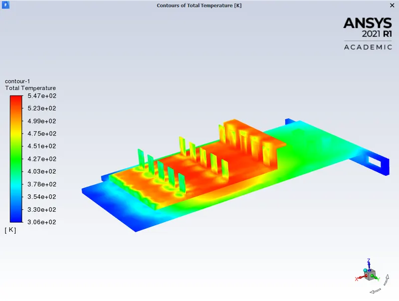
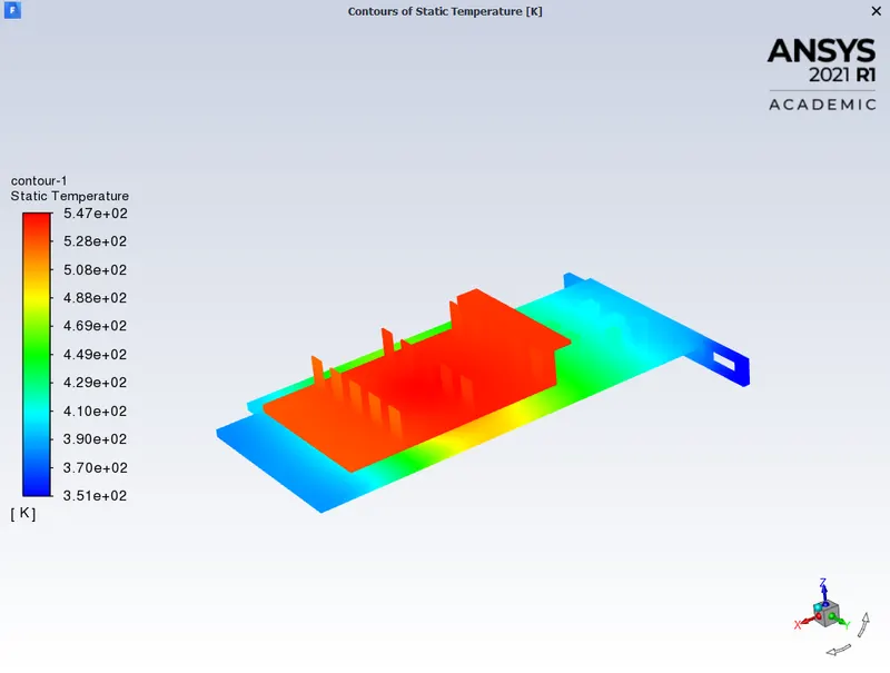
Total temperature:
Static temperature:
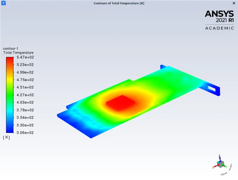
The total temperature at base:
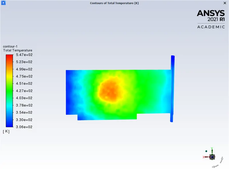
The total temperature at the bottom face of the base:
Potential hotspot at base:
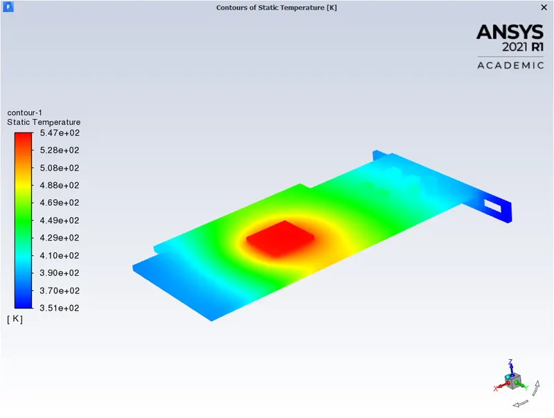
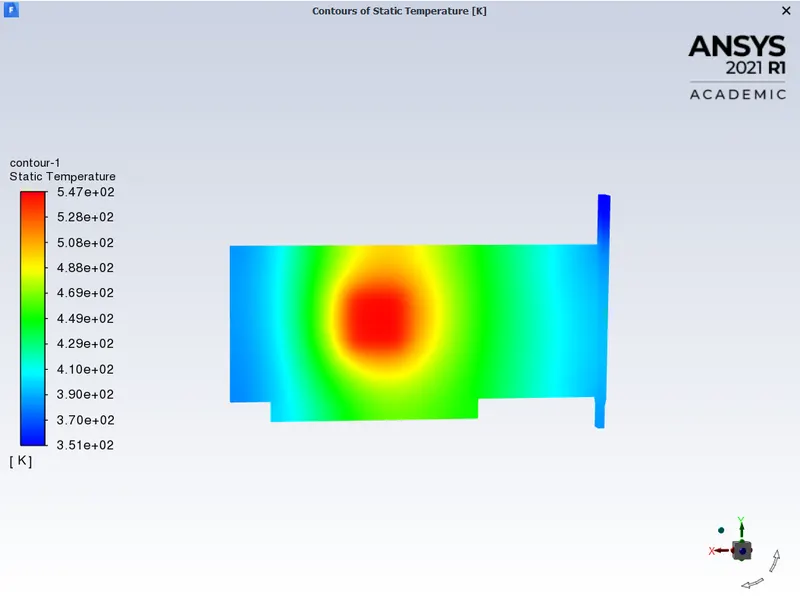
Potential hotspot at the bottom face of the base:
The total temperature at fins:
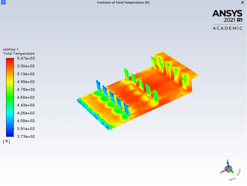
The total temperature at the bottom face of the fins:
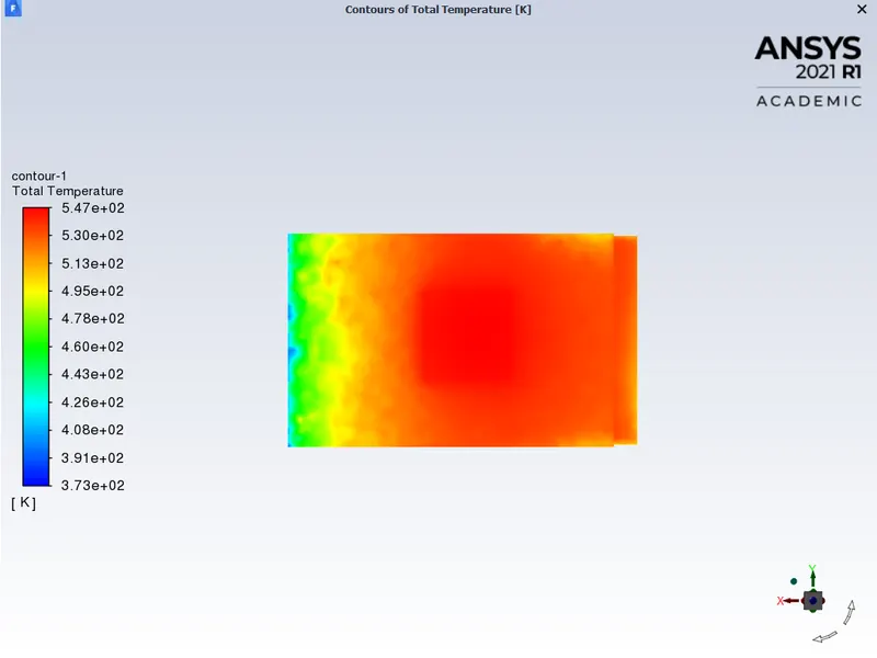
Potential hotspot at fins:
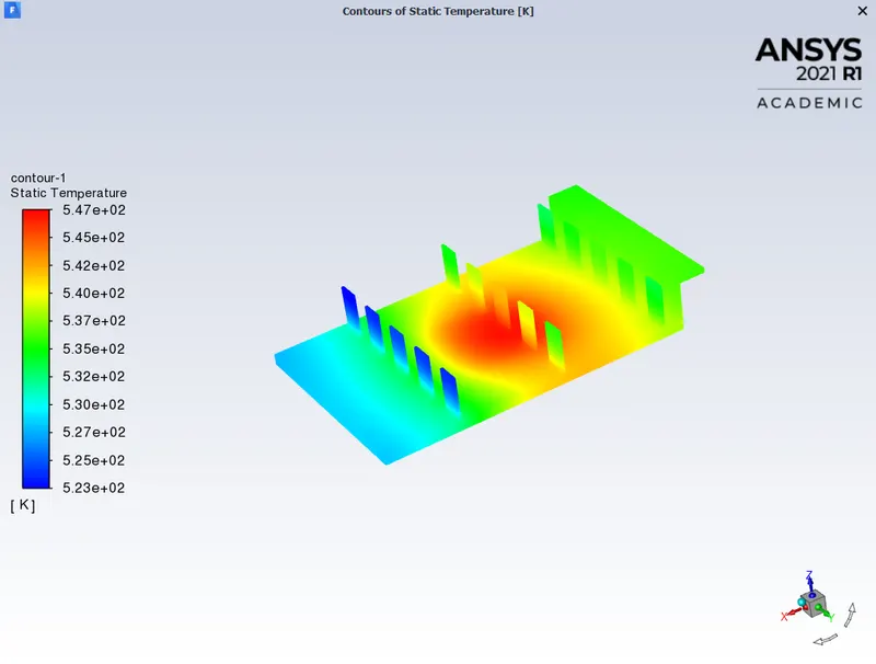
Potential hotspot at the bottom face of the fins:
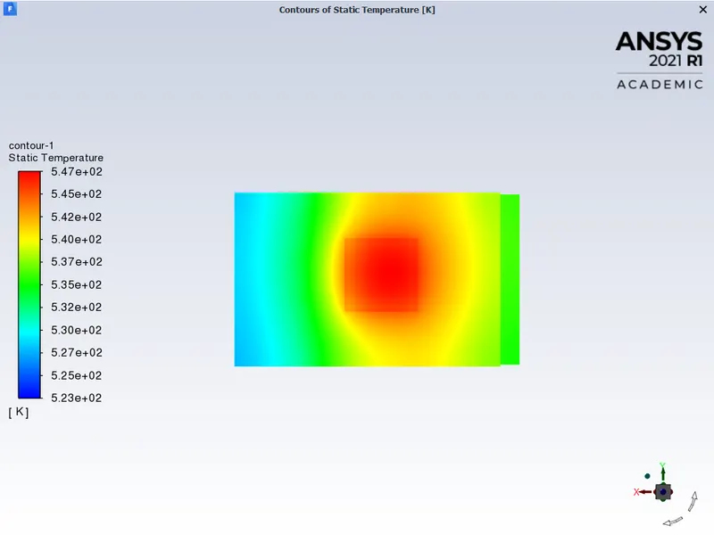
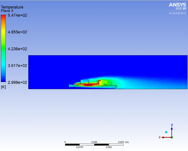
The temperature at the processor:
The maximum temperature at the processor is 547.4193 K
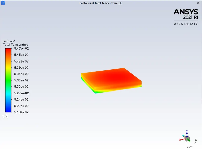
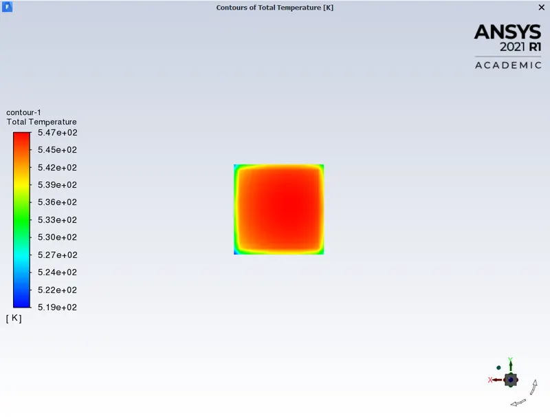
The temperature at the bottom face of the processor:
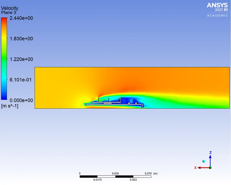
Velocity contour at XZ plane where y=0:
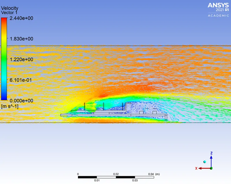
Velocity vector:
Temperature contour at XZ plane where y=0:
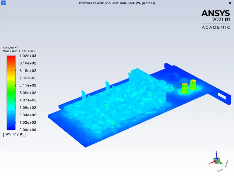
Wall HTC at graphics card:
The maximum value of the Wall heat transfer coefficient is `1018.135 W/(m^2K)`
Wall HTC at fins:
The maximum value of the Wall heat transfer coefficient at fins is `497.6152 W/(m^2K)`
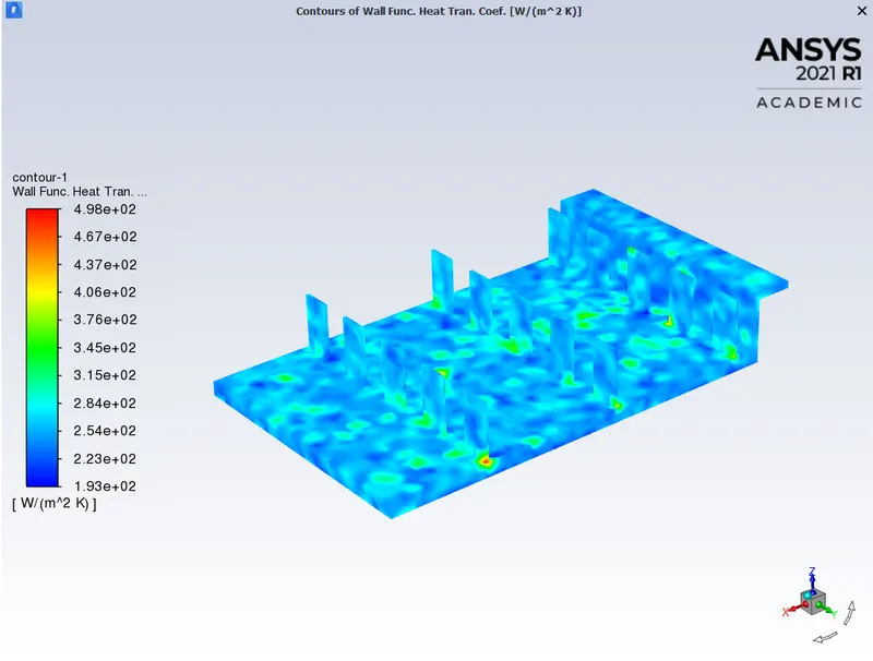
Wall HTC at processor:
The maximum value of the Wall heat transfer coefficient at the processor is `533.4137 W/(m^2K)`
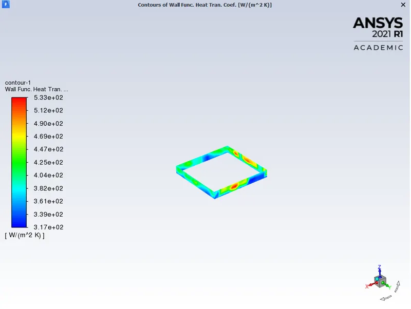
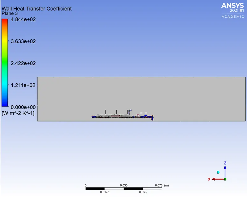
Wall HTC at XZ plane where y=0:
The maximum value of the Wall heat transfer coefficient is `484.413 W/(m^2K)`
Case 3:
Velocity = 3 m/s
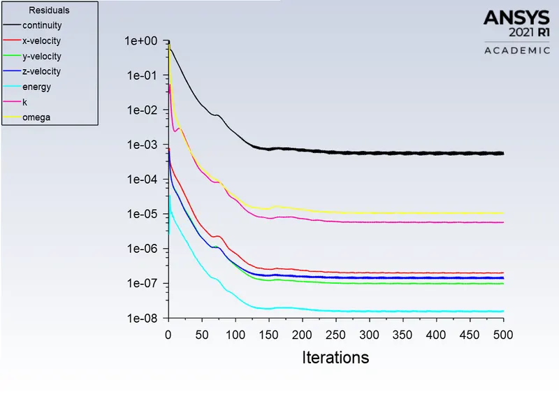
Residual plot:
From the residual plot, as shown below, the solution can be considered as converged as the variation of residuals is less and follows the same pattern. It can be said that the solution is converged around 200 iterations.
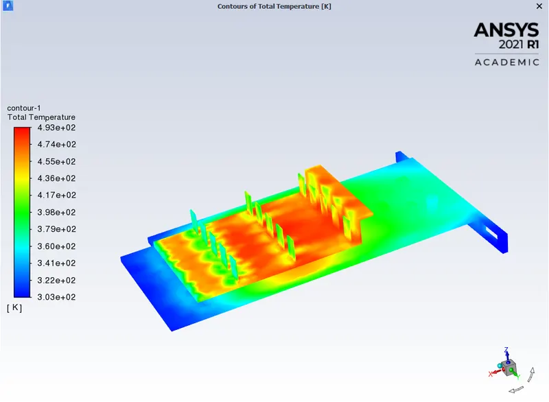
Total temperature:
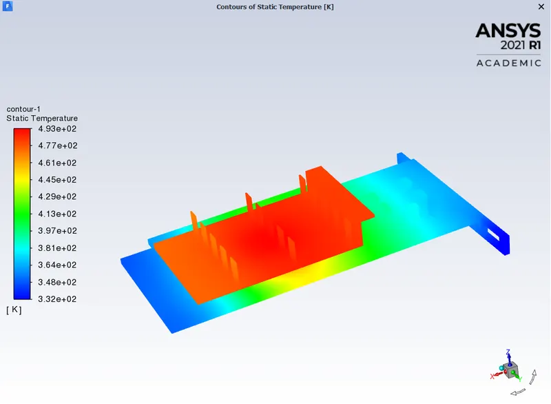
Static temperature:
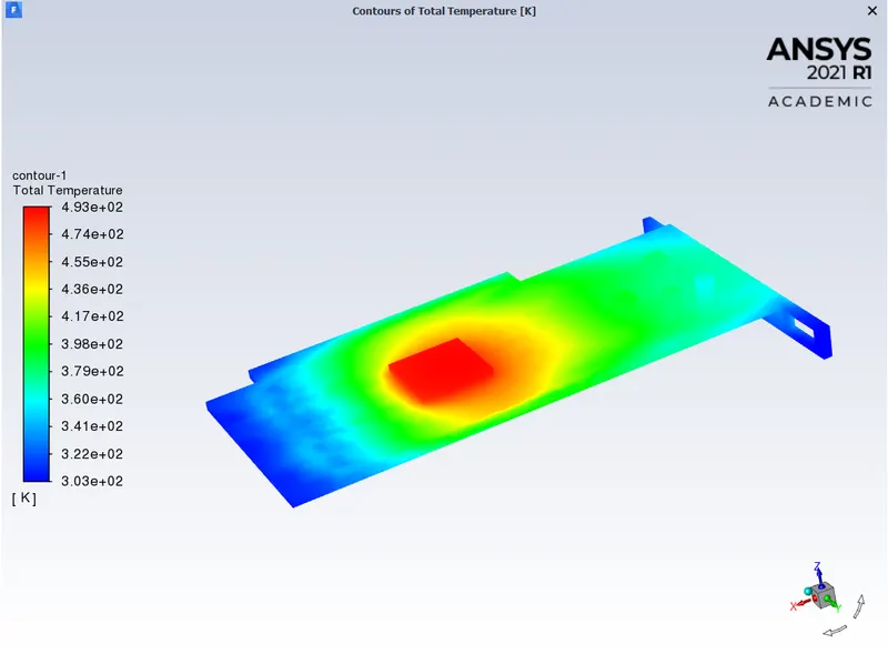
The total temperature at base:
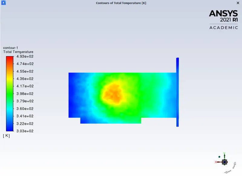
The total temperature at the bottom face of the base:
Potential hotspot at base:
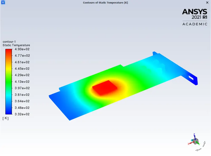
Potential hotspot at the bottom face of the base:
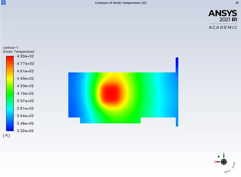
The total temperature at fins:
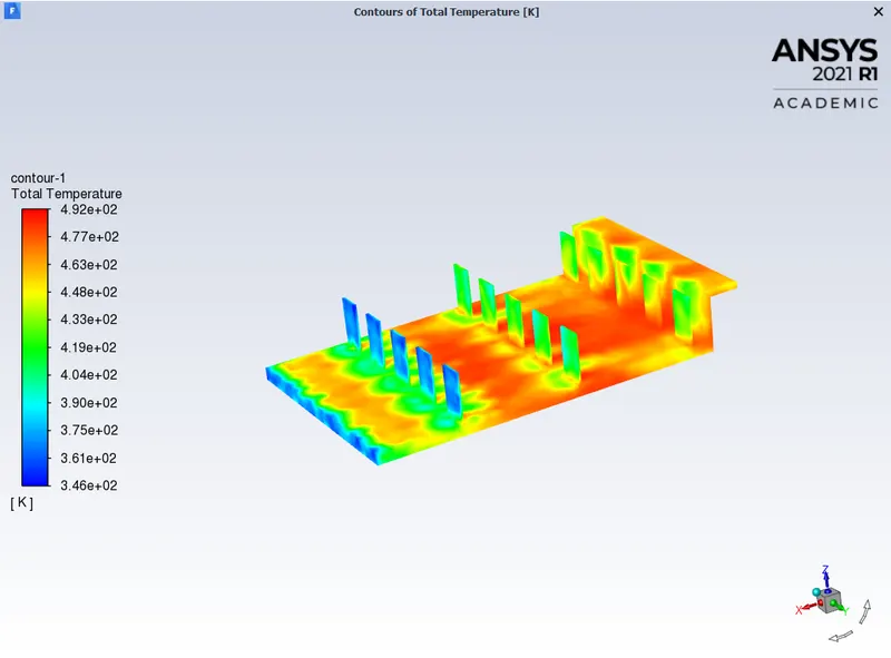
The total temperature at the bottom face of the fins:
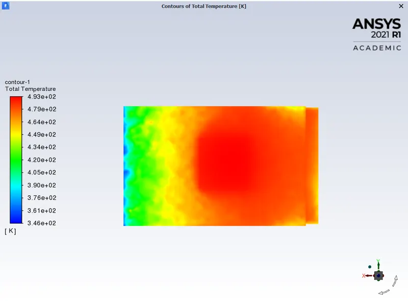
Potential hotspot at fins:
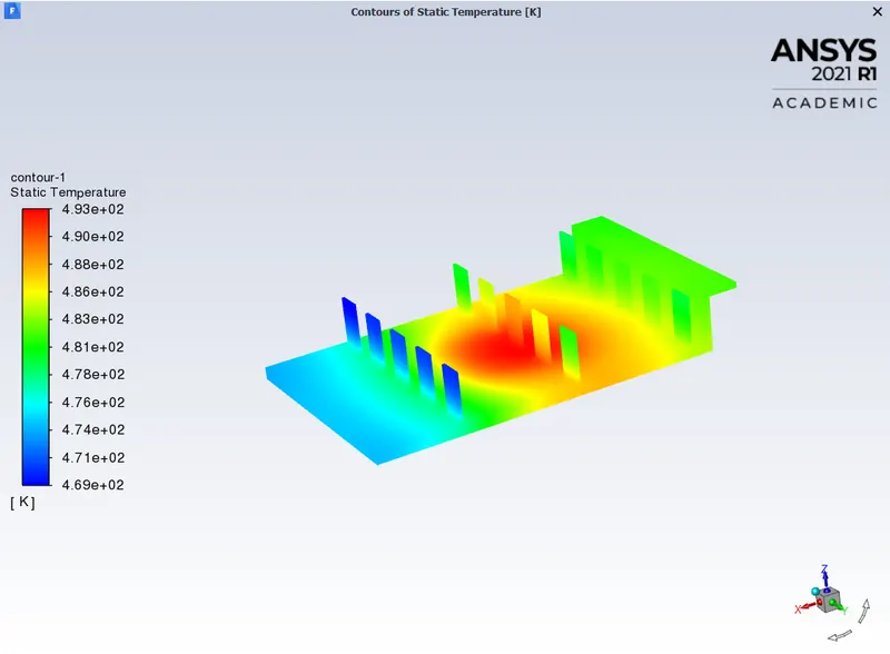
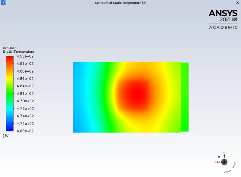
Potential hotspot at the bottom face of the fins:
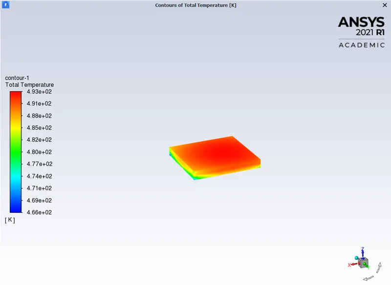
The temperature at the processor:
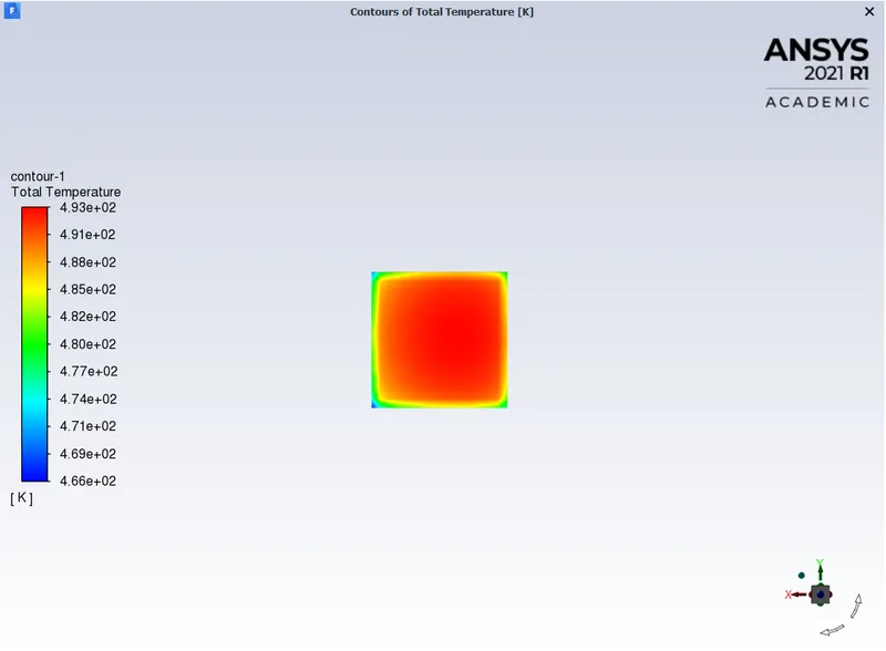
The maximum temperature at the processor is 493.4896 K
The temperature at the bottom face of the processor:
Velocity contour at XZ plane where y=0:
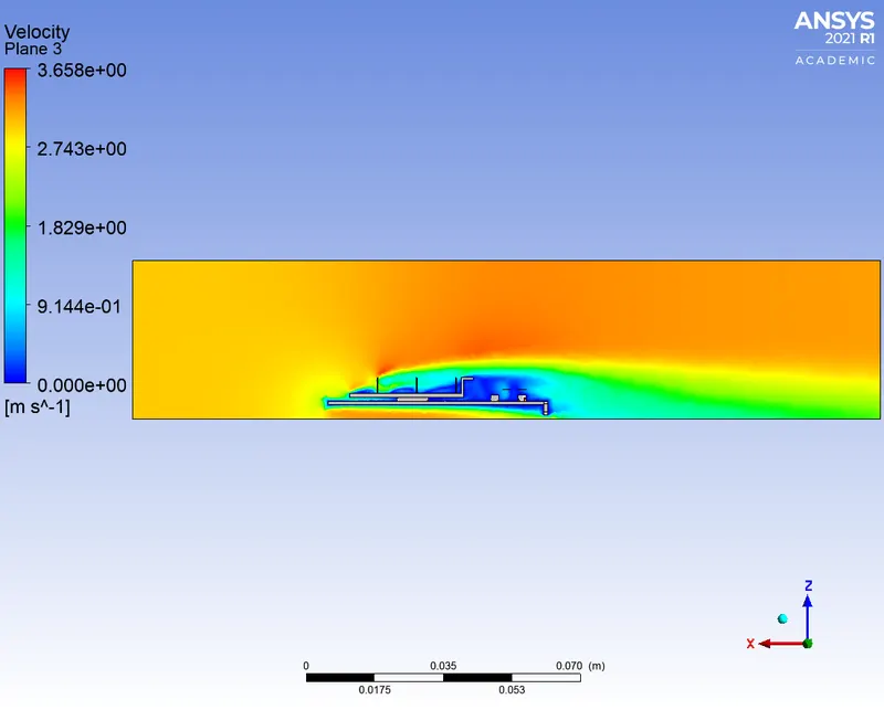
Velocity vector:
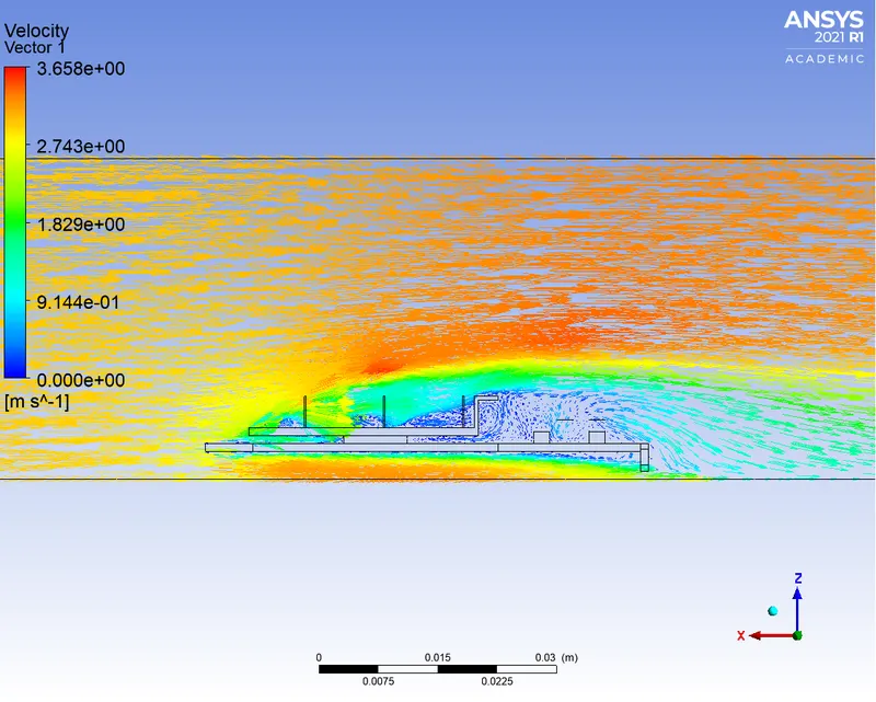
Temperature contour at XZ plane where y=0:
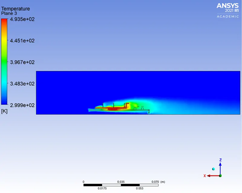
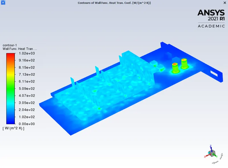
Wall HTC at graphics card:
The maximum value of the Wall heat transfer coefficient is `1018.142 W/(m^2K)`
Wall HTC at fins:
The maximum value of the Wall heat transfer coefficient at fins is `500.8317 W/(m^2K)`
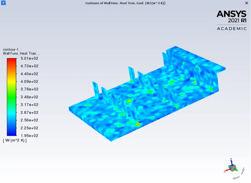
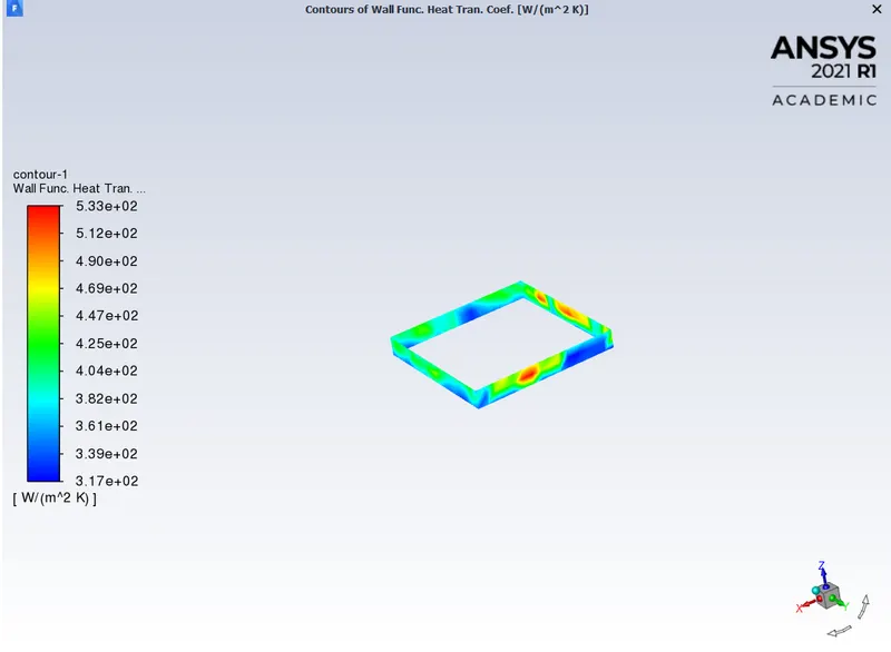
Wall HTC at processor:
The maximum value of the Wall heat transfer coefficient at the processor is `533.4147 W/(m^2K)`
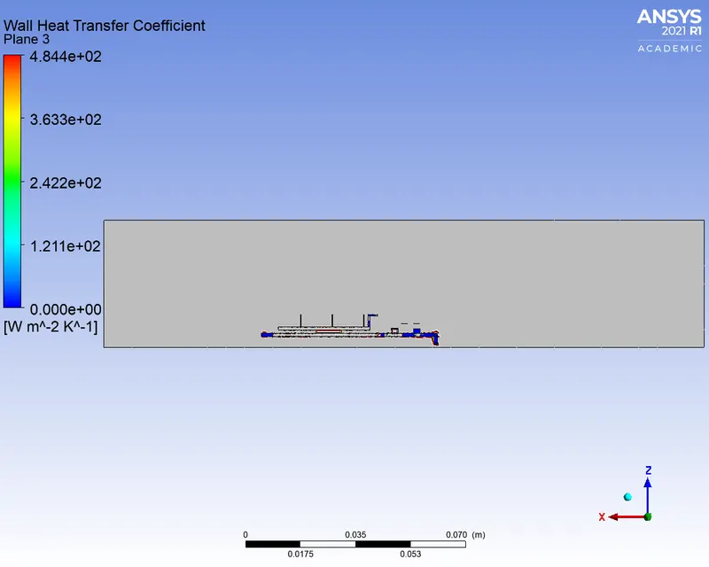
Wall HTC at XZ plane where y=0:
The maximum value of the Wall heat transfer coefficient is `484.413 W/(m^2K)`
Case 4:
Velocity = 4 m/s
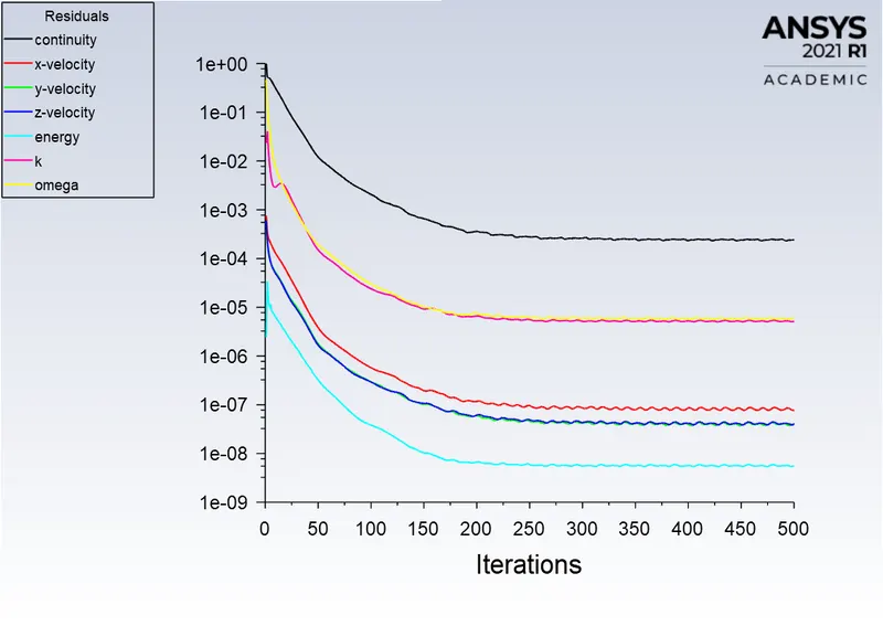
Residual plot:
From the residual plot, as shown below, the solution can be considered as converged as the variation of residuals is less and follows the same pattern. It can be said that the solution is converged around 225 iterations.
Total temperature:
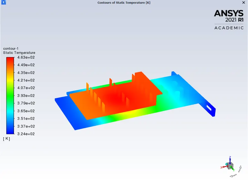
Static temperature:
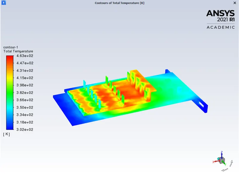
The total temperature at base:
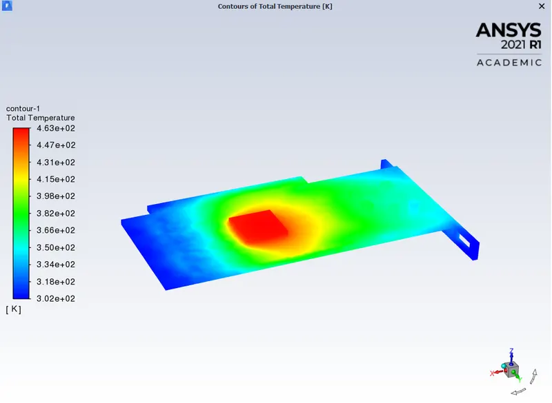
The total temperature at the bottom face of the base:
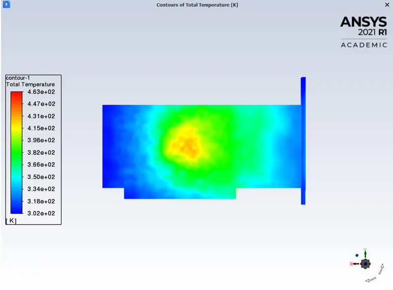
Potential hotspot at base:
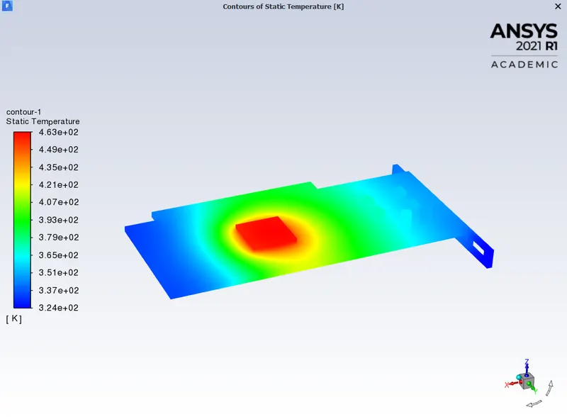
Potential hotspot at the bottom face of the base:
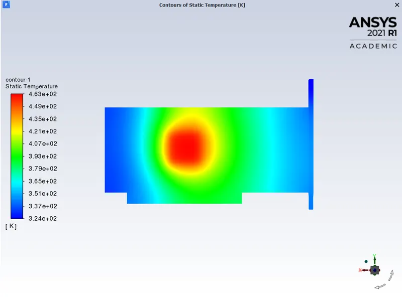
The total temperature at fins:
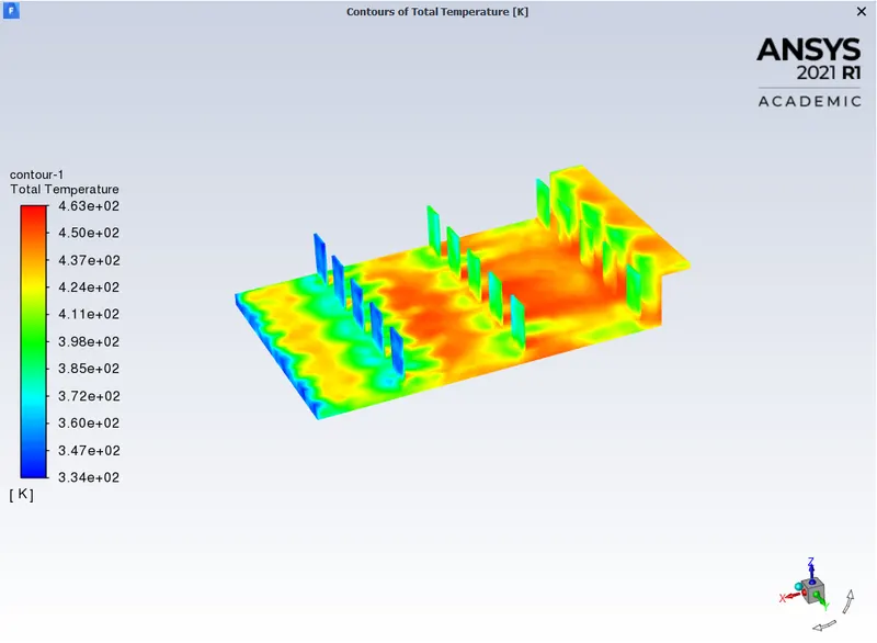
The total temperature at the bottom face of the fins:
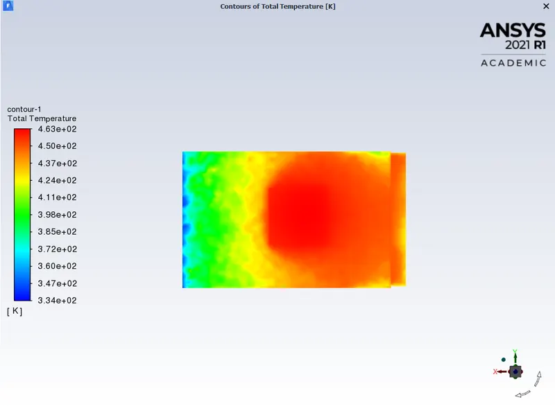
Potential hotspot at fins:
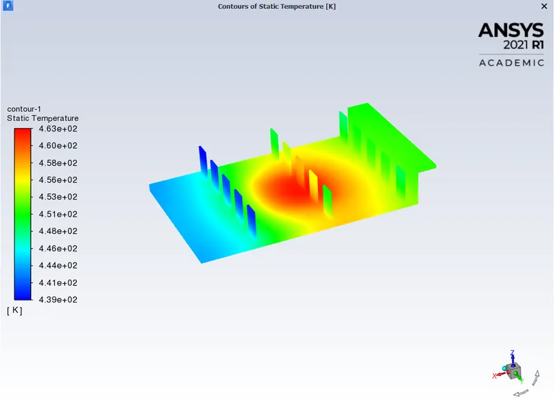
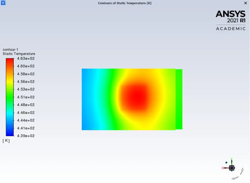
Potential hotspot at the bottom face of the fins:
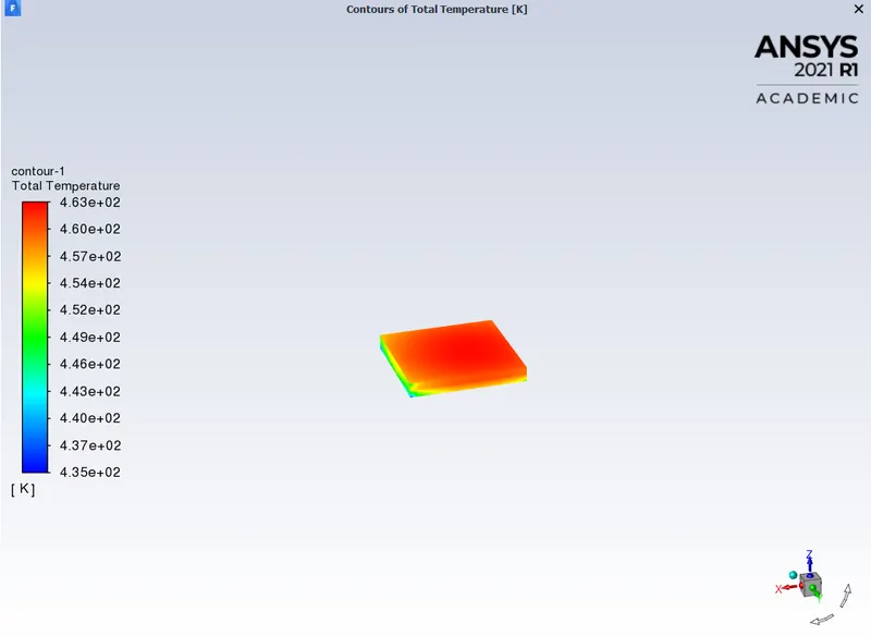
The temperature at the processor:
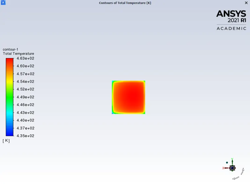
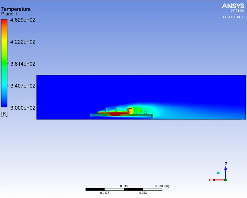
The maximum temperature at the processor is 462.9798 K
The temperature at the bottom face of the processor:
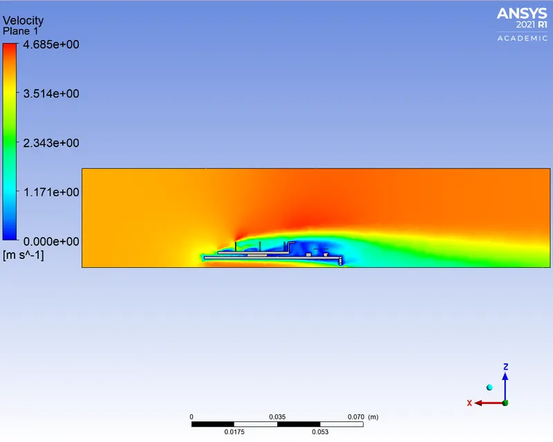
Velocity contour at XZ plane where y=0:
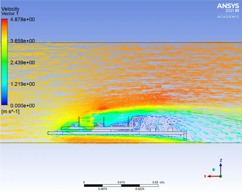
Velocity vector:
Temperature contour at XZ plane where y=0:
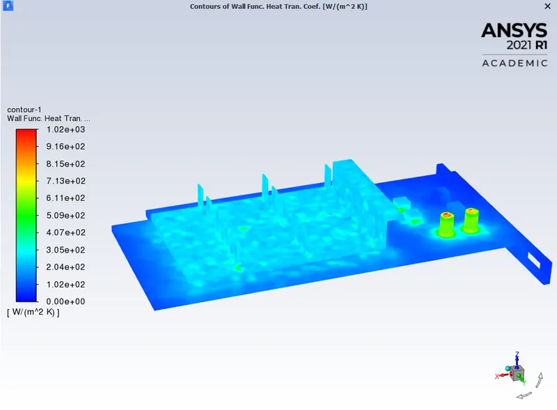
Wall HTC at graphics card:
The maximum value of the Wall heat transfer coefficient is `1018.164 W/(m^2K)`
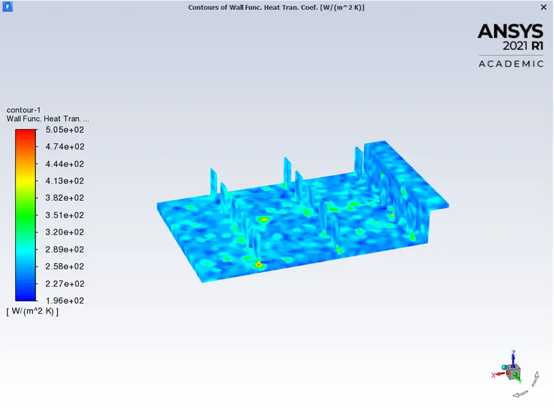
Wall HTC at fins:
The maximum value of the Wall heat transfer coefficient at fins is `505.3575 W/(m^2K)`
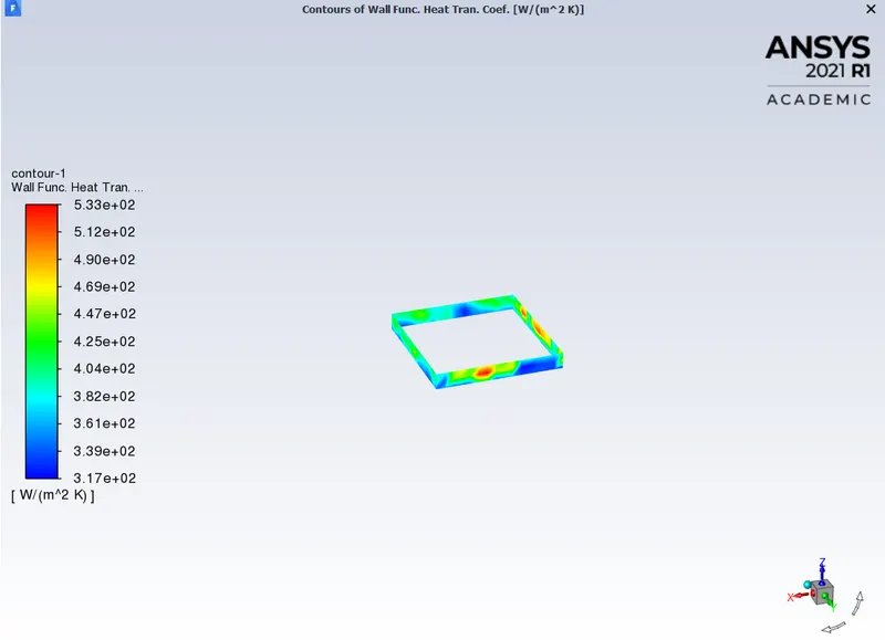
Wall HTC at processor:
The maximum value of the Wall heat transfer coefficient at the processor is `533.422 W/(m^2K)`
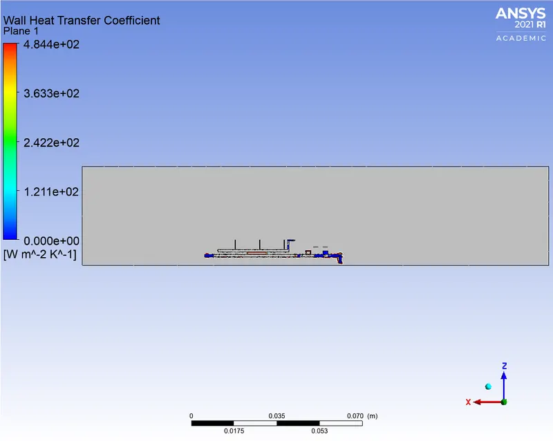
Wall HTC at XZ plane where y=0:
The maximum value of the Wall heat transfer coefficient is `484.413 W/(m^2K)`
Case 5:
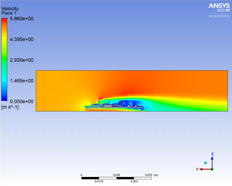
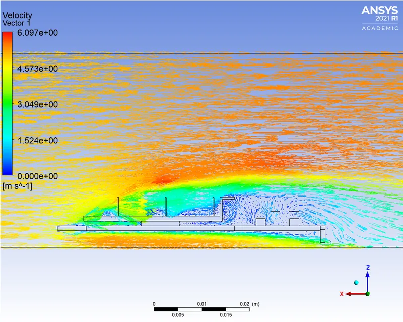
Velocity = 5 m/s
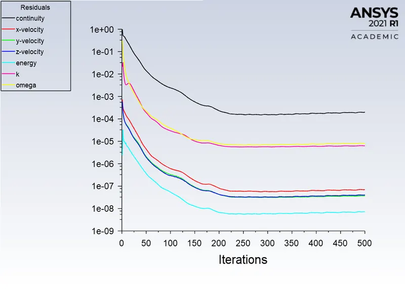
Residual plot:
From the residual plot, as shown below, the solution can be considered as converged as the variation of residuals is less and follows the same pattern. It can be said that the solution is converged around 225 iterations.
Total temperature:
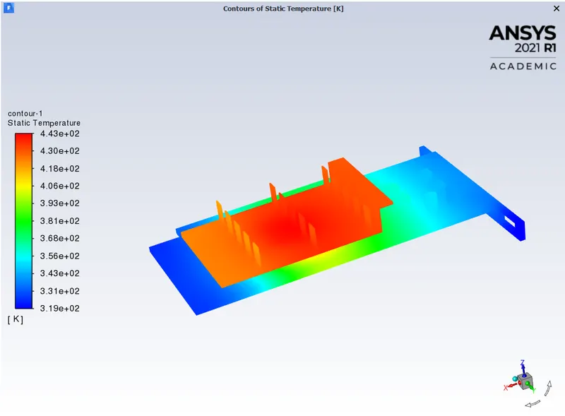
Static temperature:
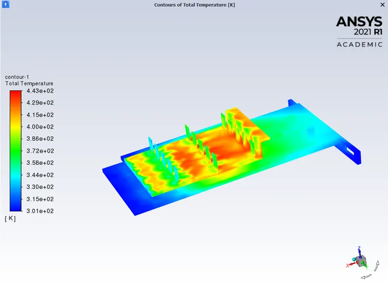
The total temperature at base:
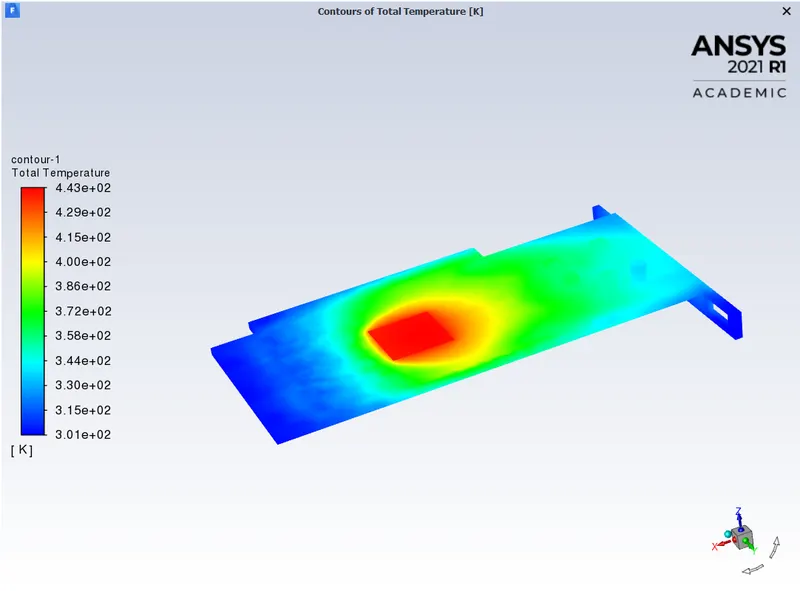
The total temperature at the bottom face of the base:
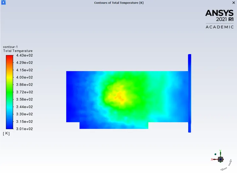
Potential hotspot at base:
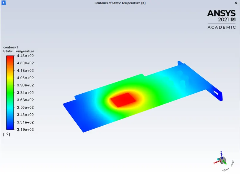
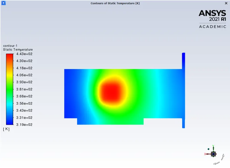
Potential hotspot at the bottom face of the base:
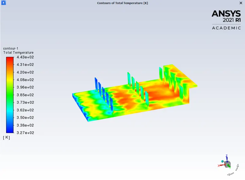
The total temperature at fins:
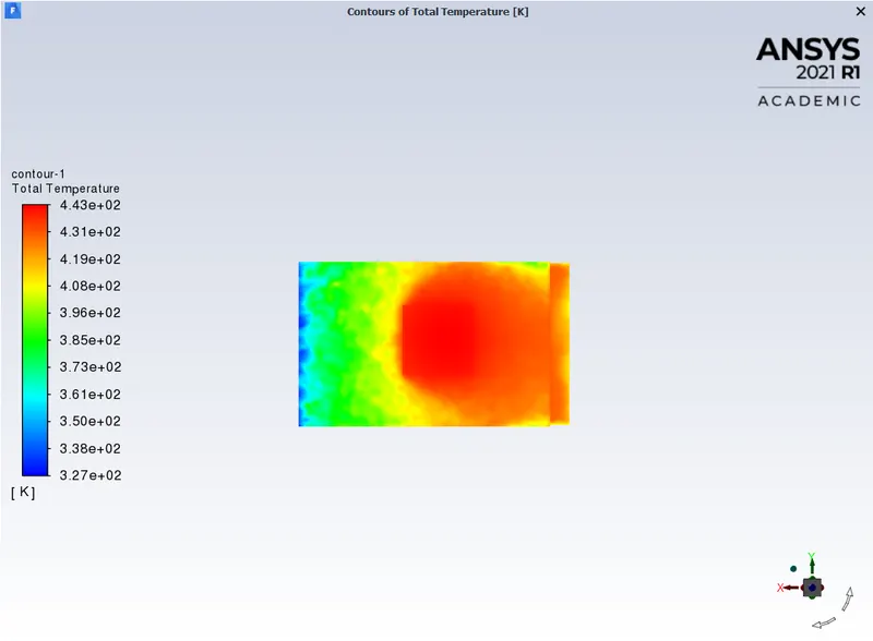
The total temperature at the bottom face of the fins:
Potential hotspot at fins:
Potential hotspot at the bottom face of the fins:
The temperature at the processor:
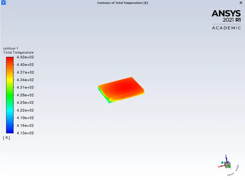
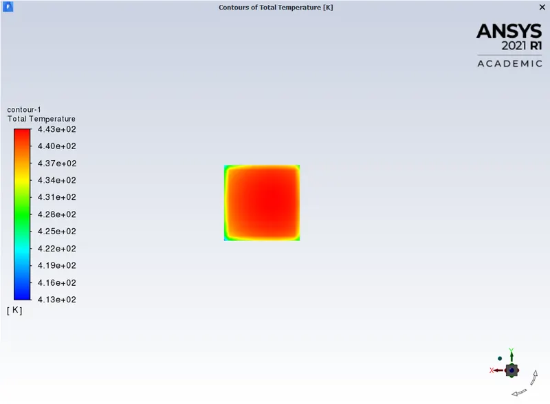
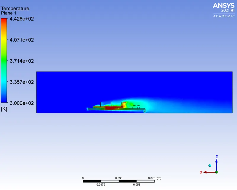
The maximum temperature at the processor is 442.8406 K
The temperature at the bottom face of the processor:
Velocity contour at XZ plane where y=0:
Velocity vector:
Temperature contour at XZ plane where y=0:
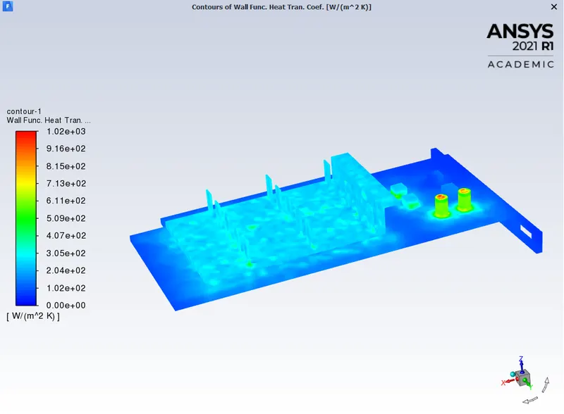
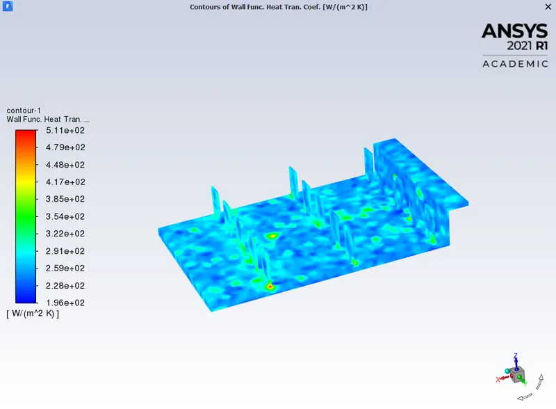
Wall HTC at graphics card:
The maximum value of the Wall heat transfer coefficient is `1018.219 W/(m^2K)`
Wall HTC at fins:
The maximum value of the Wall heat transfer coefficient at fins is `510.9528 W/(m^2K)`
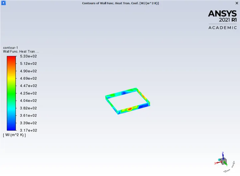
Wall HTC at processor:
The maximum value of the Wall heat transfer coefficient at the processor is `533.4334 W/(m^2K)`
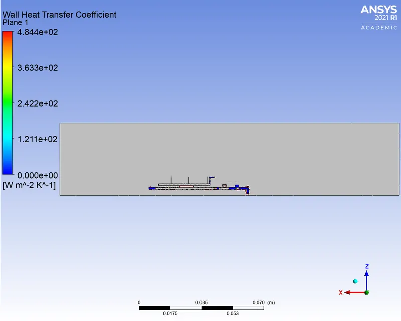
Wall HTC at XZ plane where y=0:
The maximum value of the Wall heat transfer coefficient is `484.414 W/(m^2K)`
Observations:
- Residual plots: The residual measures the local imbalance of a conserved variable in each control volume. Therefore, every cell in the model has its own residual value for the equations being solved. The solution can be considered as converged as the variation of residuals are less or change is very small and follows the same pattern. In our case, it can be said that the solution is converged after 125 iterations for case 1, 150 iterations for case 2, 200 iterations for case 3, 225 iterations for case 4, and 225 iterations for case 5.
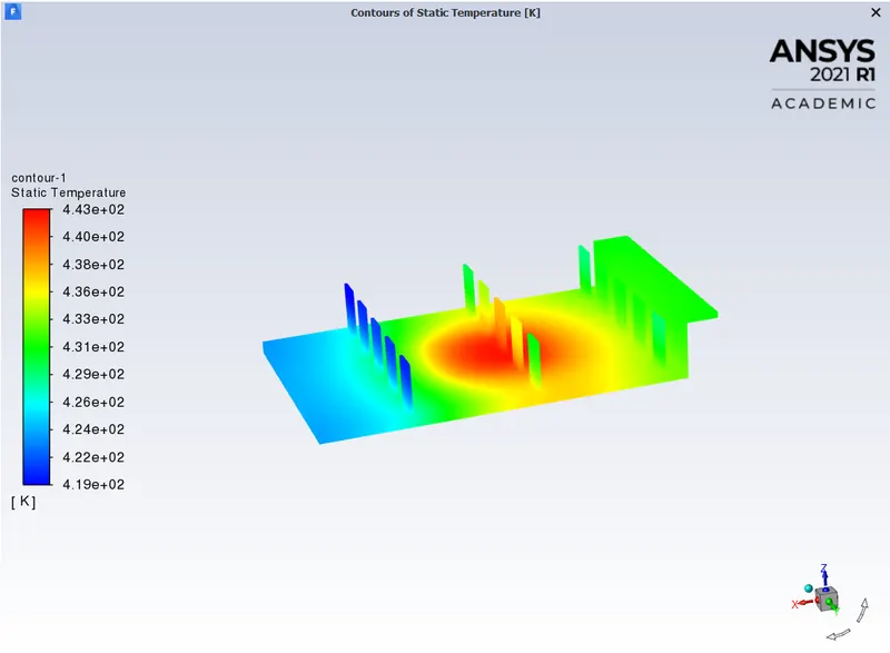
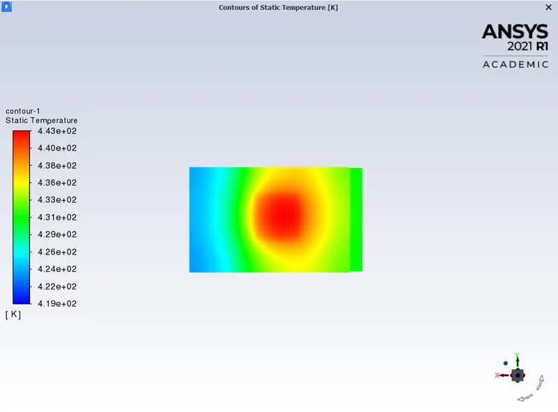
- Temperature plots: From the temperature plots, we can see hotspots in the fin and base near the surface that is in contact with the processor because it is only the area that generates heat during the working of the graphics card. The high-temperature regions are found at the center of the fins, base, and processor walls. Conduction occurred between processor and fins, and processor and base. Convection occurred when the heat generated is removed by the inlet airflow.
- As we increased the velocity of air from 1m/s to 5m/s the temperature of fins decreased because the convective heat transfer increases.
- In the refined case the temperature distribution is accurate and the heat transfer coefficient increases.
| Inlet Velocity (m/s) | Mesh | Max Temperature at Processor (K) | Max Wall Heat Transfer Coefficient at Processor `(W/(m^2 K))` |
| 1 | Baseline | 665.8619 | 78.1379 |
| 1 | Refined | 681.3875 | 533.4125 |
| 2 | Refined | 547.4191 | 533.4137 |
| 3 | Refined | 493.4896 | 533.4147 |
| 4 | Refined | 462.9798 | 533.4220 |
| 5 | Refined | 442.8406 | 533.4334 |
- From the above table, it is clear that the maximum heat transfer coefficient is obtained when the velocity is equal to 5m/s and also the processor temperature is minimum when the velocity is equal to 5m/s.
- With the increase in velocity, the temperature dropped from 681 K at 1m/s to 442 K at 5m/s.
- We can say higher the velocity higher is the heat dissipated from the graphics card which helps in decreasing the temperature of the processor.
Conclusions:
- The maximum temperature observed in the graphics card is inversely proportional to the inlet fluid velocity.
- The higher the velocity higher is the heat dissipated from the graphic card.
- As the velocity of airflow increases Heat transfer coefficient increases.
- High-velocity cooling air can be an effective mode for heat dissipation.