Week 1- Mixing Tee

OBJECTIVE:

To set up steady-state simulations to compare the mixing effectiveness when hot inlet temperature is `36^o C` & the cold inlet is at `19^o C`, In the created two versions of the mixing tee. One of them is longer than the other.

Case 1

• Short mixing tee with a hot inlet velocity of 3 m/s.
• Momentum ratio of 2, 4.

Case 2

• Long mixing tee with a hot inlet velocity of 3 m/s.
• Momentum ratio of 2, 4.

In a table, compare the following values from the 2 cases.

1. Cell count
2. Average outlet temperature
3. Number of iterations for convergence

Expected results

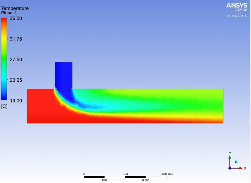
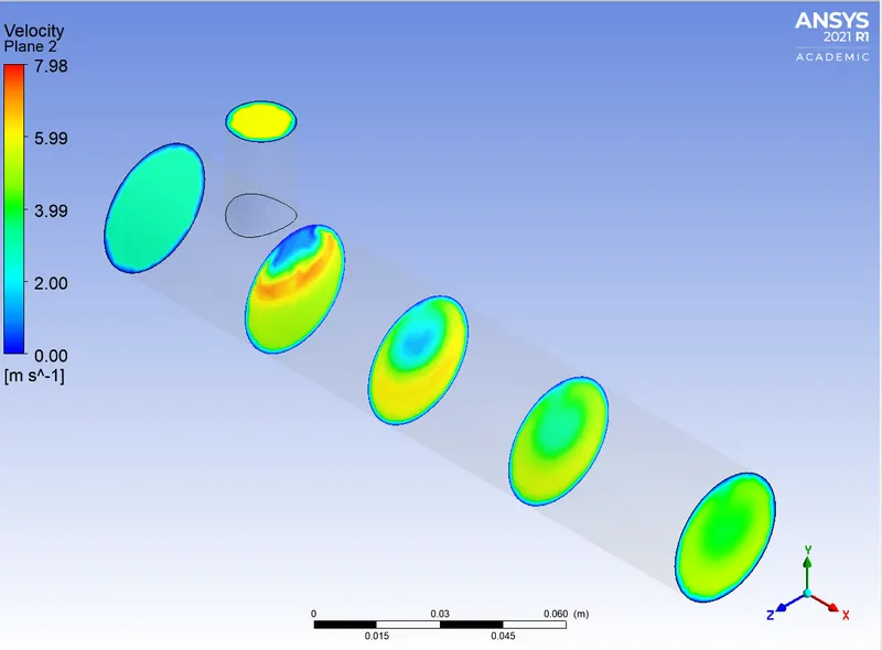
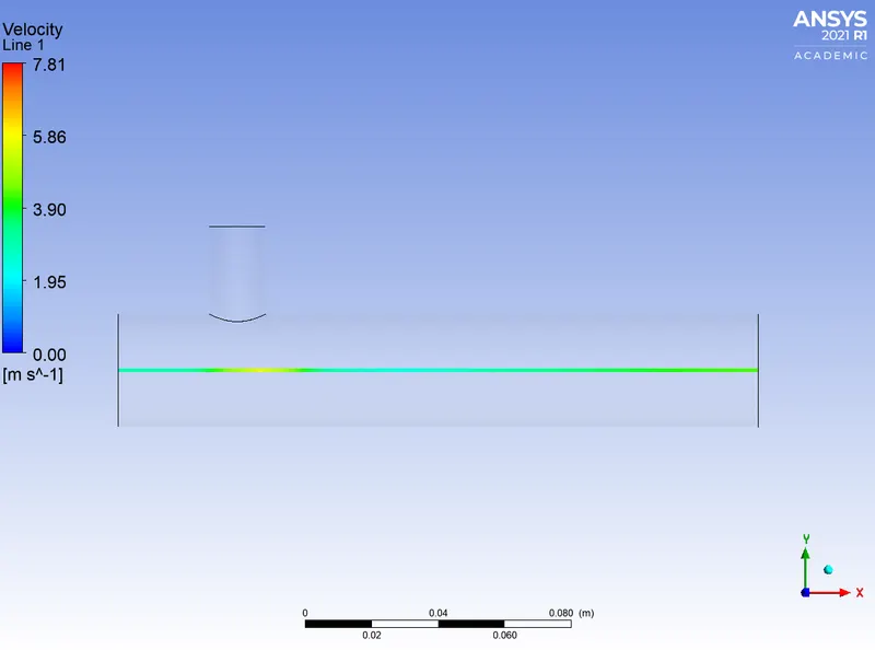
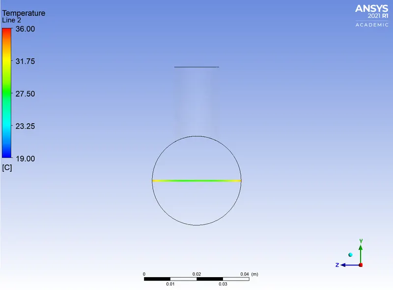
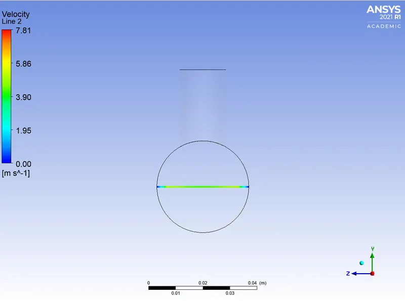
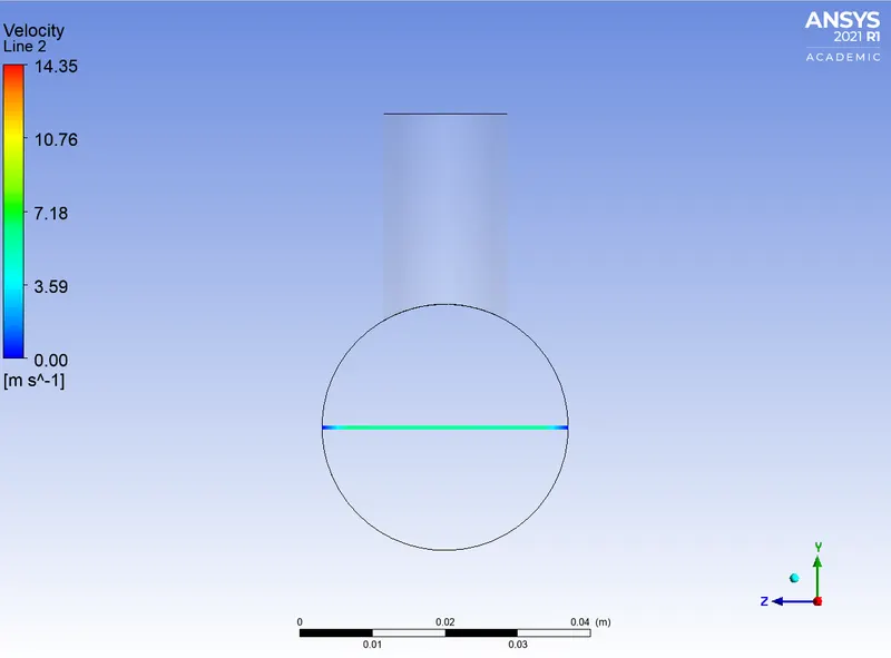
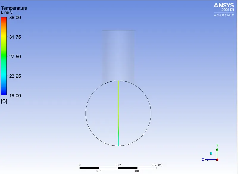
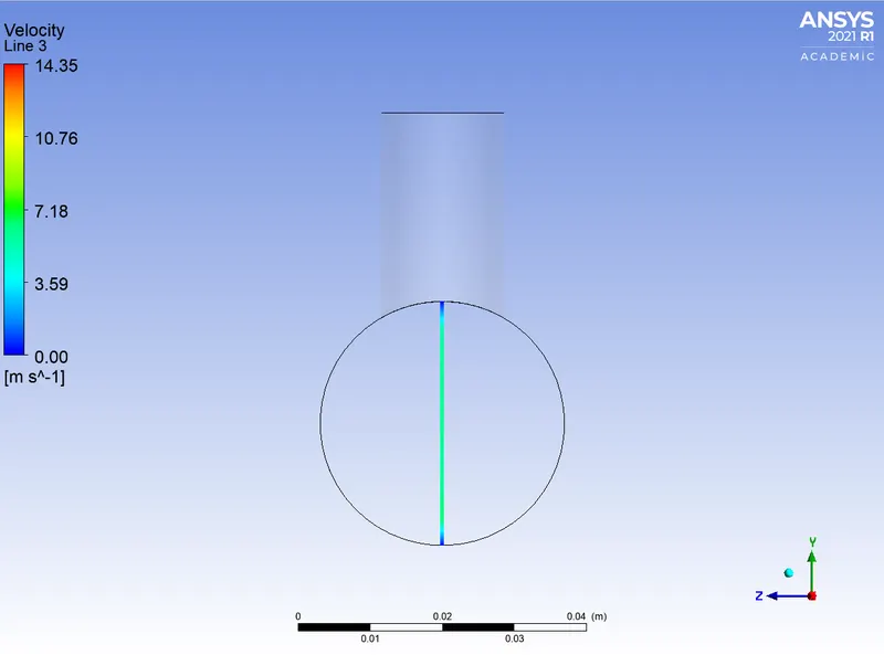
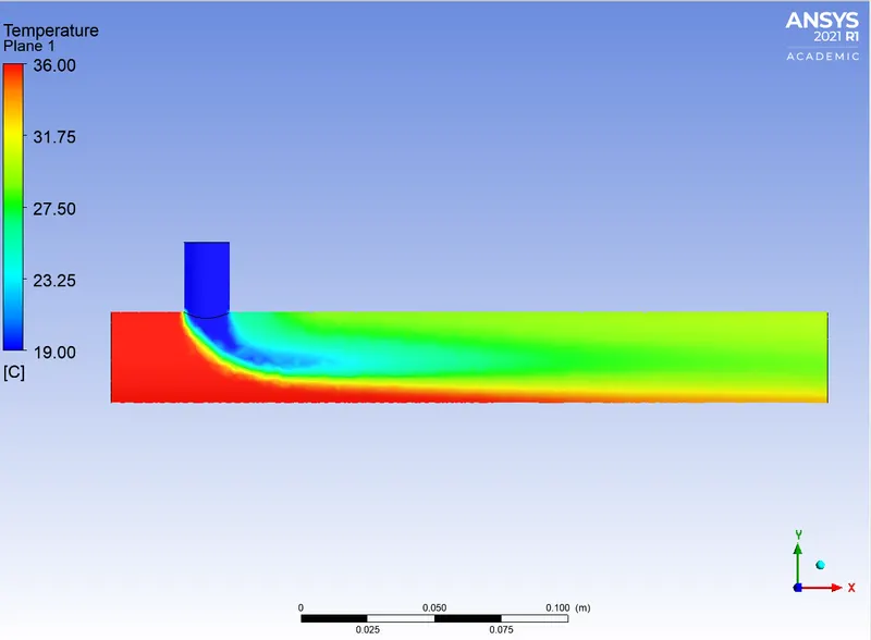
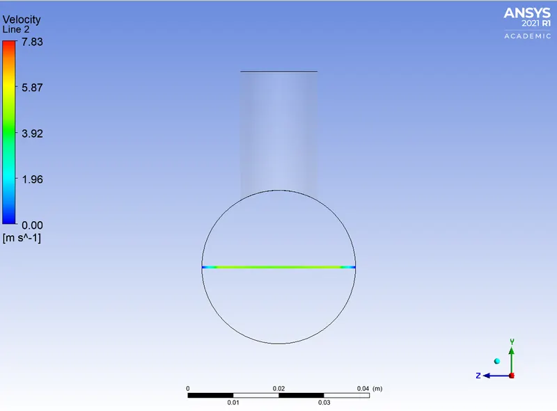
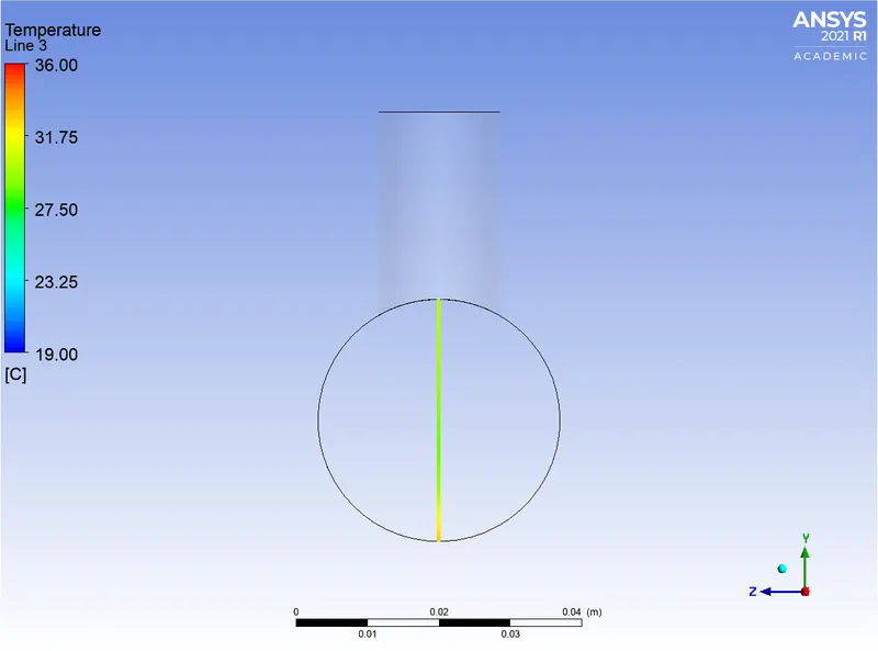
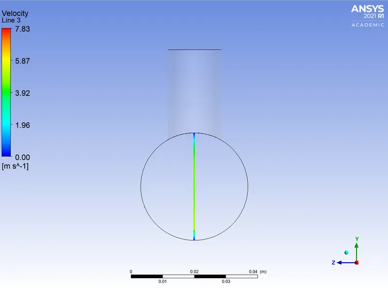
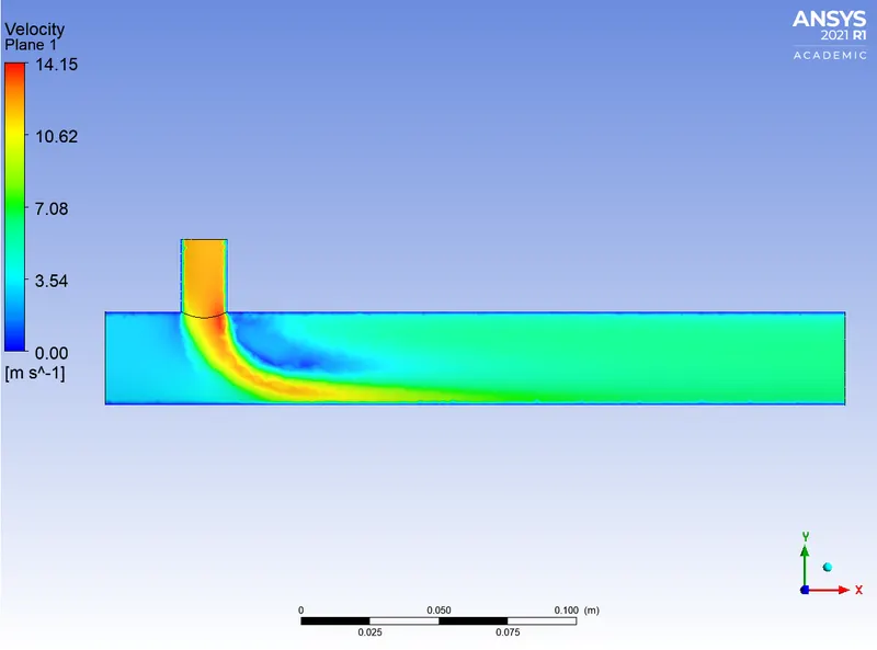
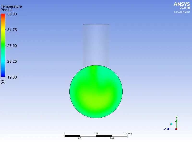
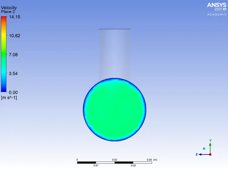
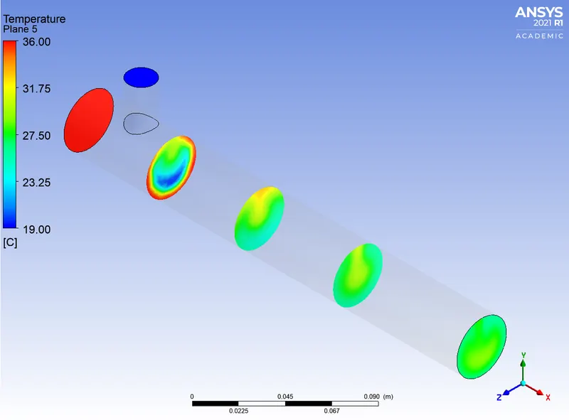
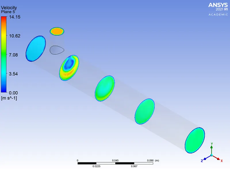
1. Velocity and temperature contour plots on the cut planes along and across the pipe.
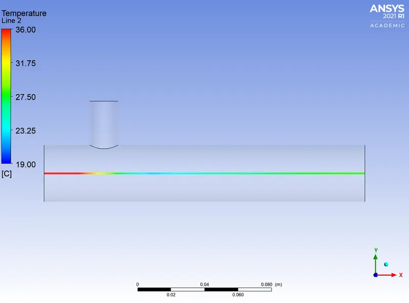
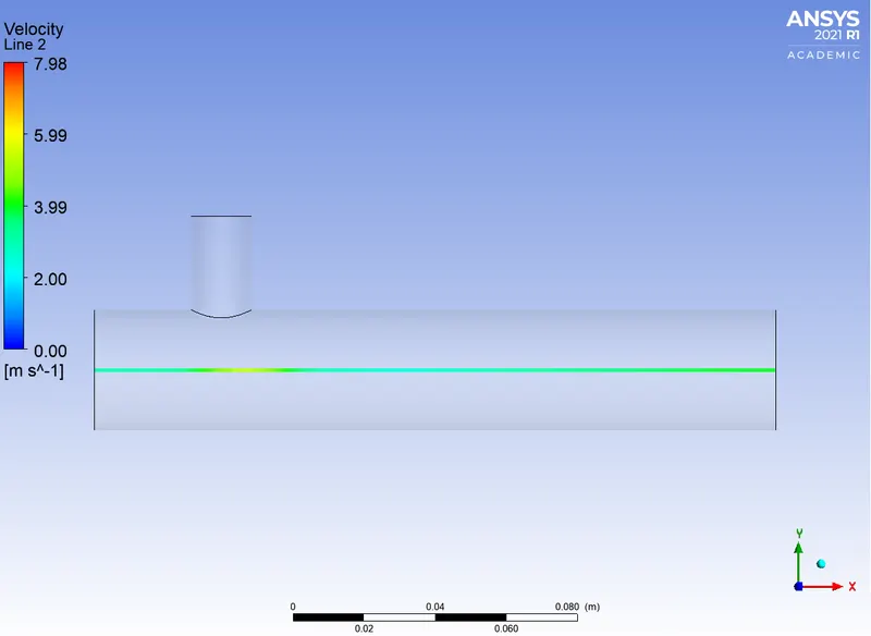
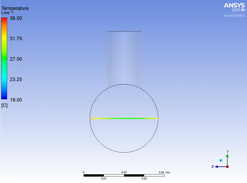
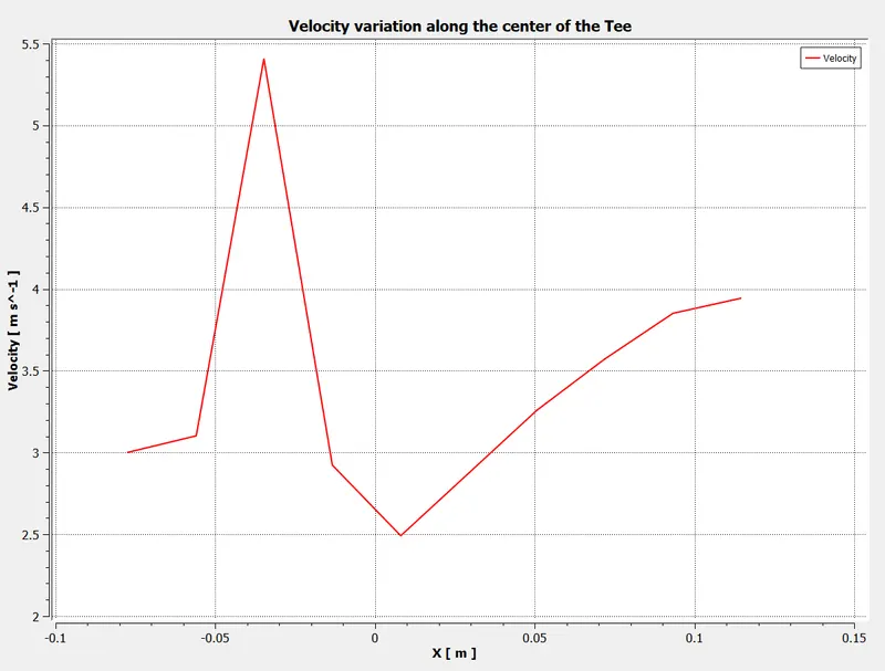
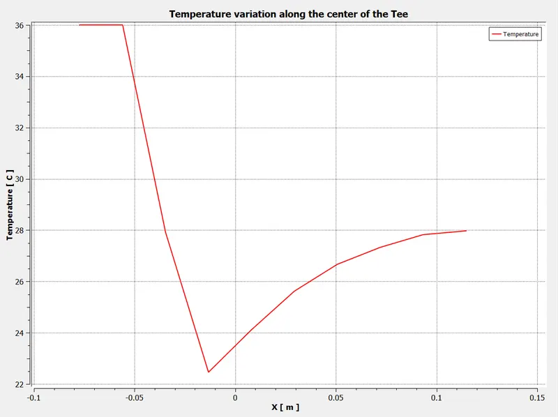
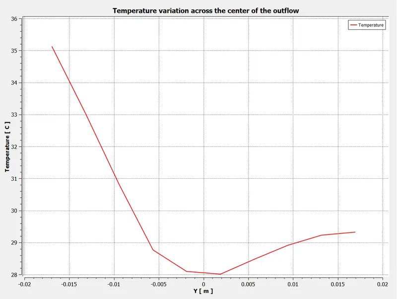
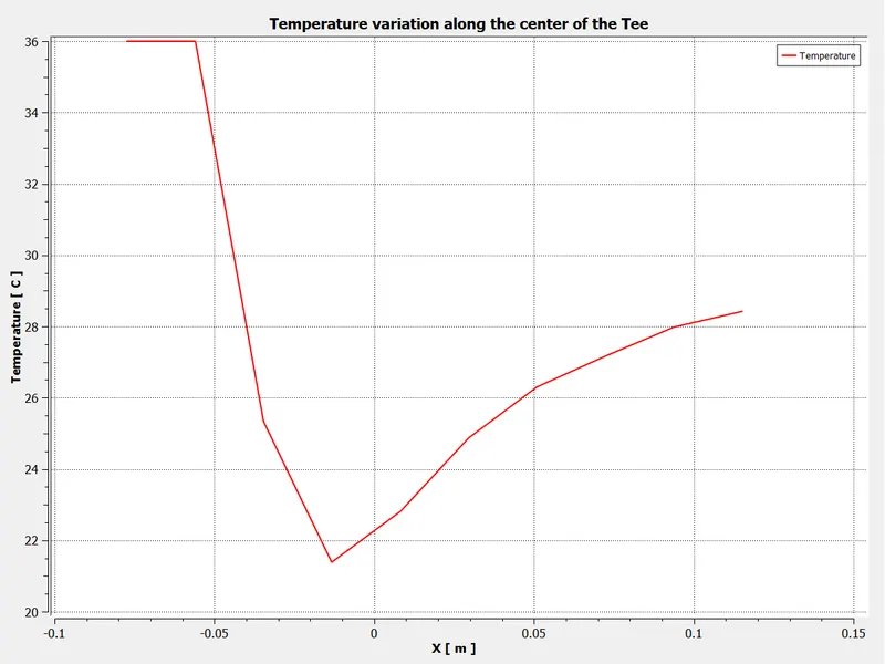
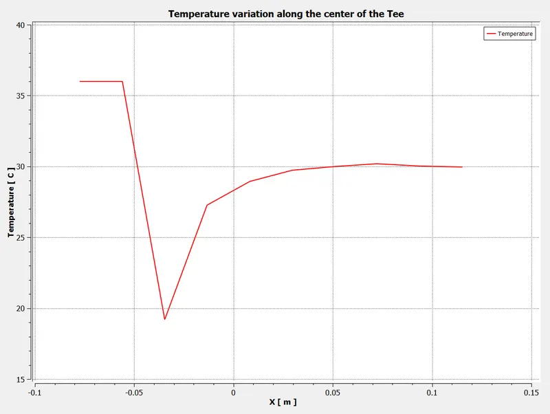
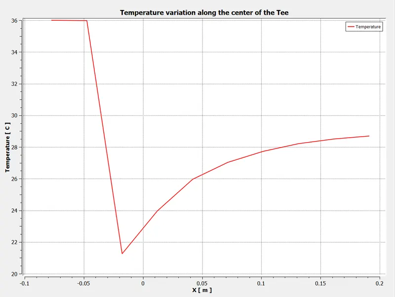
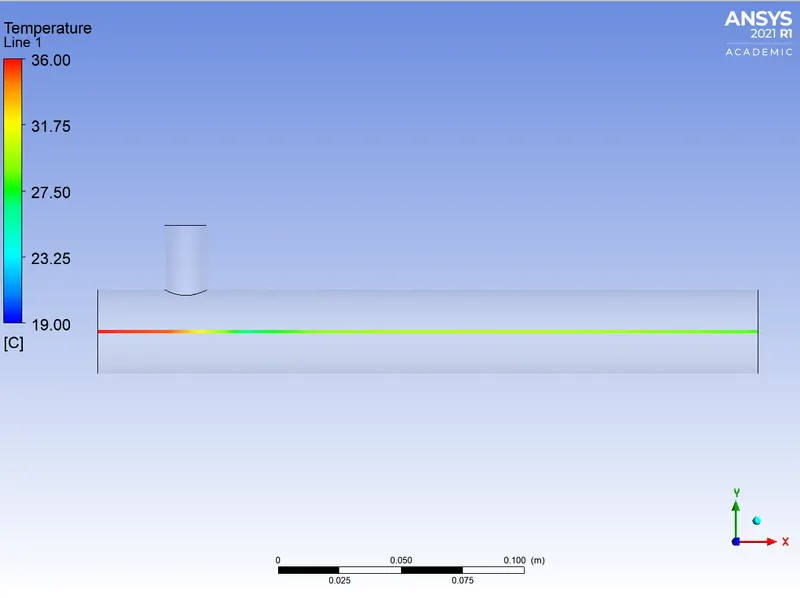
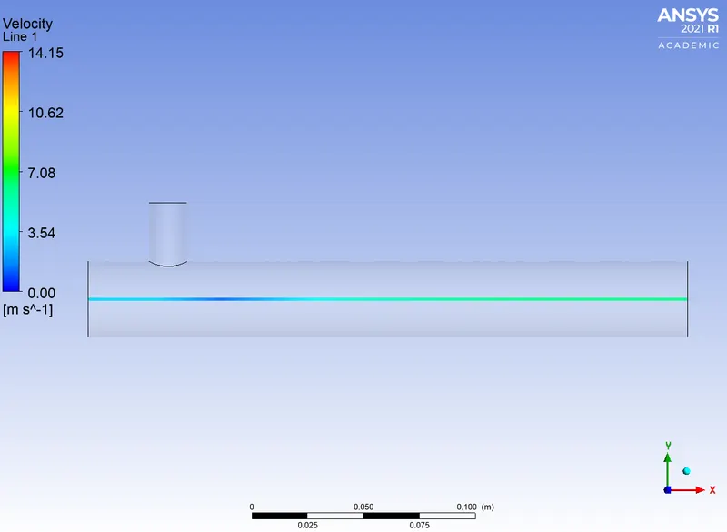
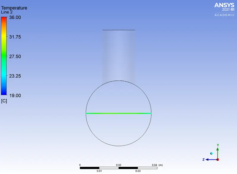
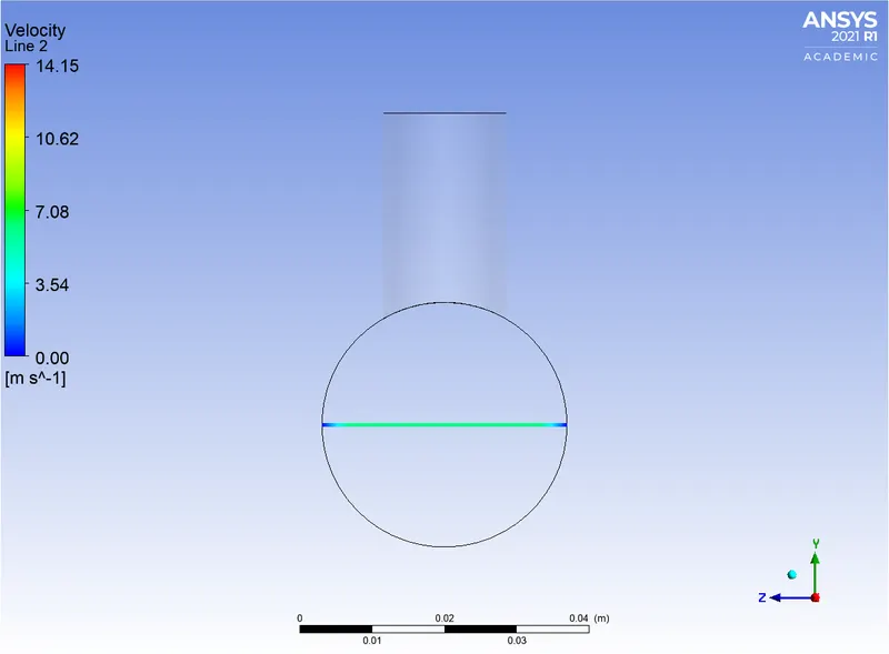
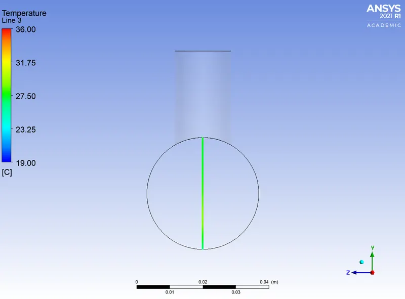
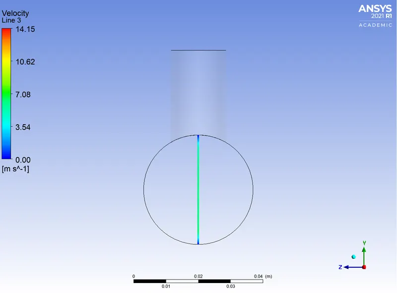
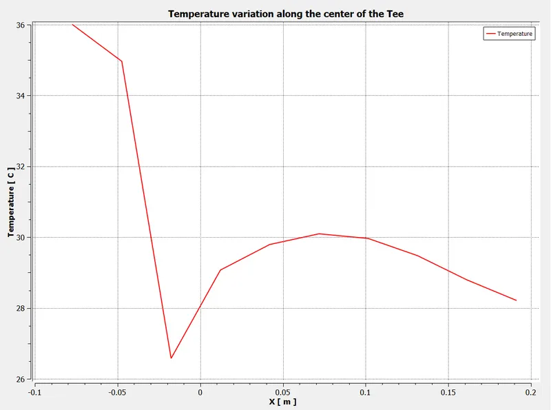
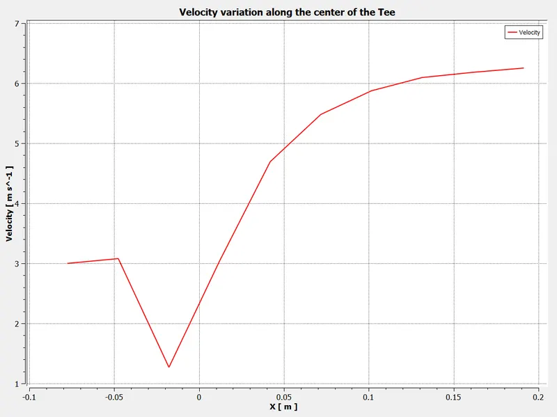
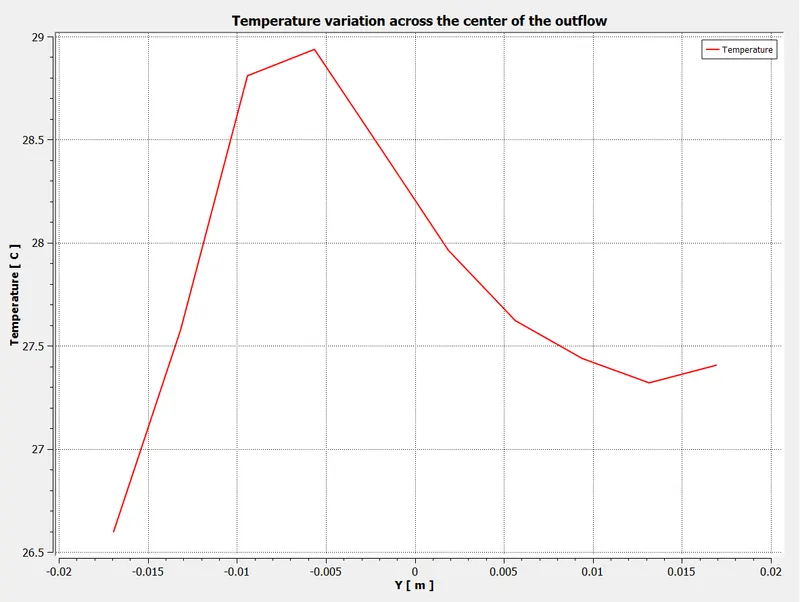
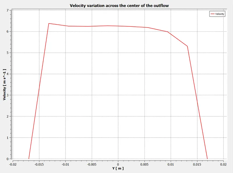
2. Velocity and temperature line plots along and across the length of the pipe.
3. Perform Mesh independent study for any one case.
4. Discuss the effect of length and momentum ratio on results.

INTRODUCTION:

A tee is formed by two pipe sections joined at a right angle to each other. The hot fluid is flowing through the main pipe while the cold fluid enters the main pipe through the branched pipe.

Concerning all the other industries, the nuclear industry is the one where the efficiency of mixing fluids in the mixing chambers is critical. There has been much research regarding the thermal stresses arising from the T-junctions due to the large temperature differences and also due to frequent changes in the same.

The temperature fluctuations cause cyclic thermal stresses and subsequent fatigue cracking of the pipe wall. Thus, anticipating the piping system's failure in nuclear power plants is essential as its failure may lead to irreparable damage. In order to assess the structural strength, stability, and life of such T-junctions, it is essential to know the magnitude of the temperature fluctuations, regions of pipe wall that experience the temperature fluctuations, the response of the material of the pipe to the thermal fatigue loading.

METHODOLOGY:

Mixing tee possesses two inlets and one outlet. The momentum ratio for this type of tee is the ratio of velocity at the cold inlet to the velocity at the hot inlet. As the mixing tee has various applications, In our case, we will be dealing with the T-joints used in Air Conditioning systems.

In this scenario, the function of the T-joint will be used to supply chilled air from the AC unit to the air-conditioned space. The air coming out from the AC system will have a much lower temperature. However, to have user-defined air temperature at the outlet, the concept of mixing-tee comes into existence.

We also have heat transfer from the fluid medium (air) to the solid pipe walls, which is nothing but Conjugate heat transfer. However, our pipe walls will be insulated so there would not be any heat transfer from the pipe wall to the surroundings. This leads to the transfer of heat again in the reverse direction (solid walls) to fluid medium (air). In this case, we are not focusing on wall effects.

As we know after two fluids interact at the mixing point, the flow conditions will become turbulent. This turbulence will ensure better mixing of hot air and cold air in the system. So it is important to resolve turbulence in a more approximate manner to get better results. So in order to resolve turbulence, we will be using Reynold's Average Navier-Stokes Equations (RANS). The solver will solve RANS equations in order to calculate flow field variables.

For the same purpose, we will use the turbulence model. In this case, we will be using two turbulence models

1. K-epsilon (Realizable)
2. K-omega (SST)

1. `k-epsilon`: The `k-epsilon` model solves for two variables: k, the turbulence kinetic energy; and `epsilon`(epsilon), the rate of dissipation on turbulence kinetic energy. Wall functions are used in this model, so the flow in the buffer region is not simulated. The `k-epsilon` model has historically been very popular for industrial applications due to its good convergence rate and relatively low memory requirements.

2. `K-omega`: The `k-omega` model is similar to the `k-epsilon` model, but it solves for `omega`(omega) - the specific rate of dissipation of kinetic energy. It is a low Reynolds number model, but it can also be used in conjunction with wall functions. It is more nonlinear, and thereby more difficult to converge than the `k-epsilon` model, and it is quite sensitive to the initial guess of the solution. The `k-omega` model is useful in many cases where the `k-epsilon` model is not accurate, such as internal flows, flows that exhibit strong curvature, separated flows, and jets.

So now we can move forward to set up the CFD case for the thermal analysis of the Mixing-Tee joint.

Steps in Simulation:

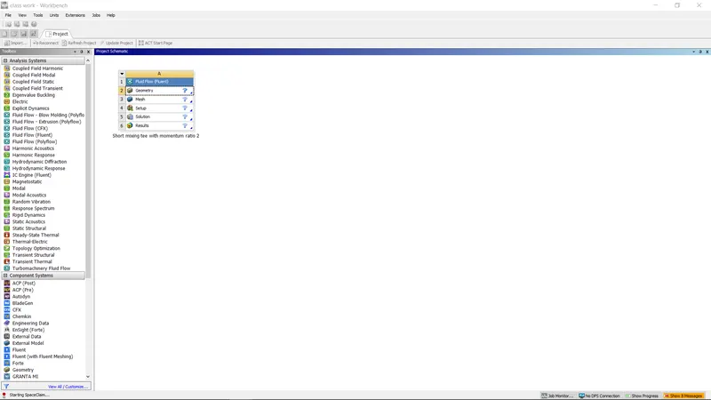
1. Open a new project, by clicking on Fluid Flow (Fluent) in the Ansys workbench.

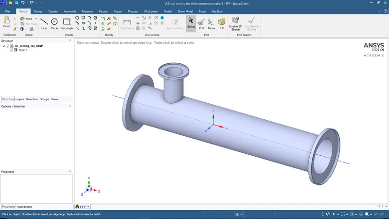
2. Now click on geometry to import the mixing tee model. It will redirect to SpaceClaim.

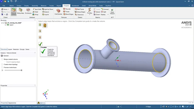
3. Now click to prepare the menu and then click on the volume extract. Switch to edge selection and select three outer edges and click on the green check button. Here we need to analyze the mixing of two fluids, so there is a role of parts other than two pipes. To suppress that we need to extract the volume of the tee.

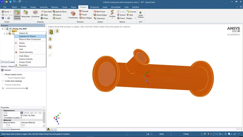
4. Hide solid by unchecking it from the structure menu to see volume, which we have extracted. Suppress solid by clicking on the option suppress for physics.

5. Then we will have Extracted volume. Then exit from SpaceClaim and click on mesh o open the mesh menu.

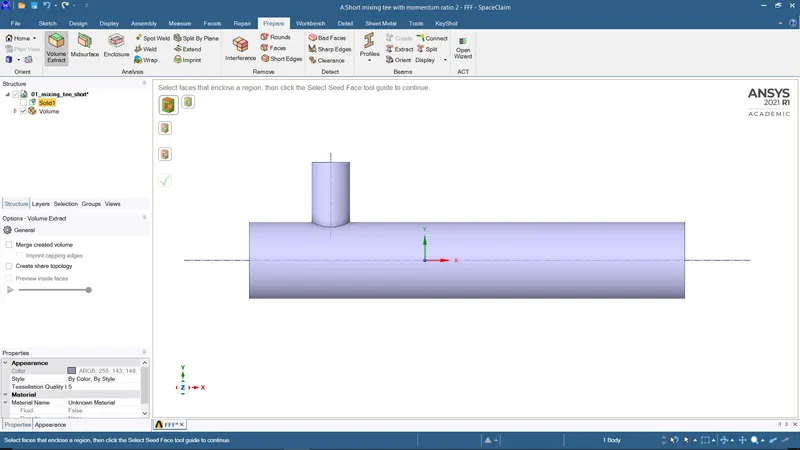
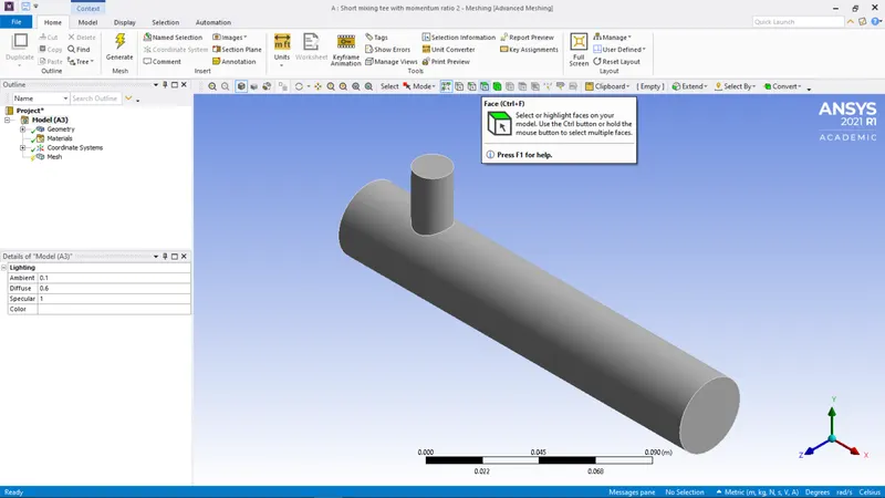
6. When the mesh window will open then press ctrl+F to select multiple faces.

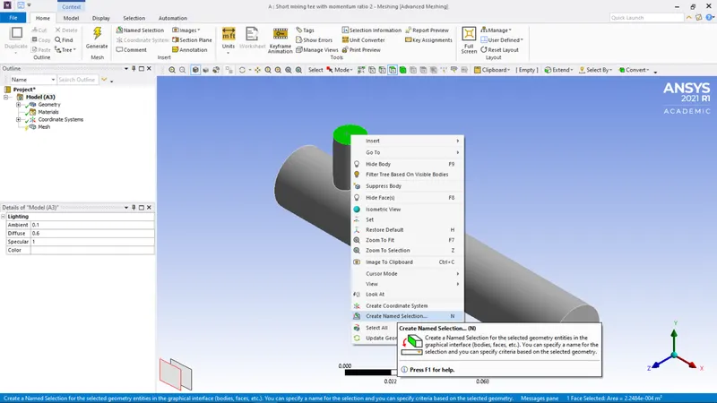
7. Select a face and press the right click of the mouse it will open a menu then click on the option create named selection and write the suitable name for face.

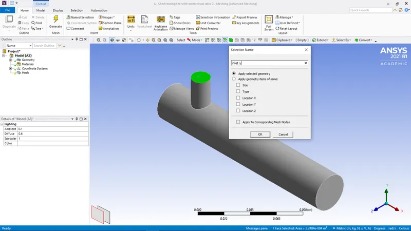
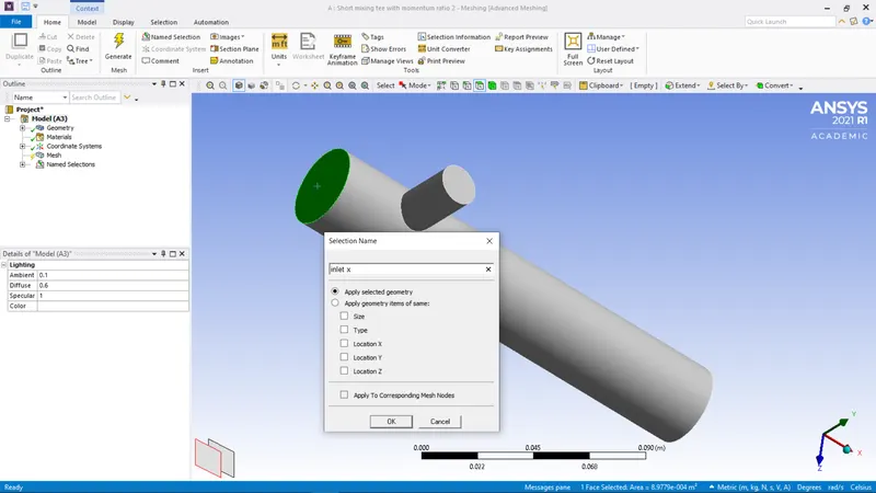
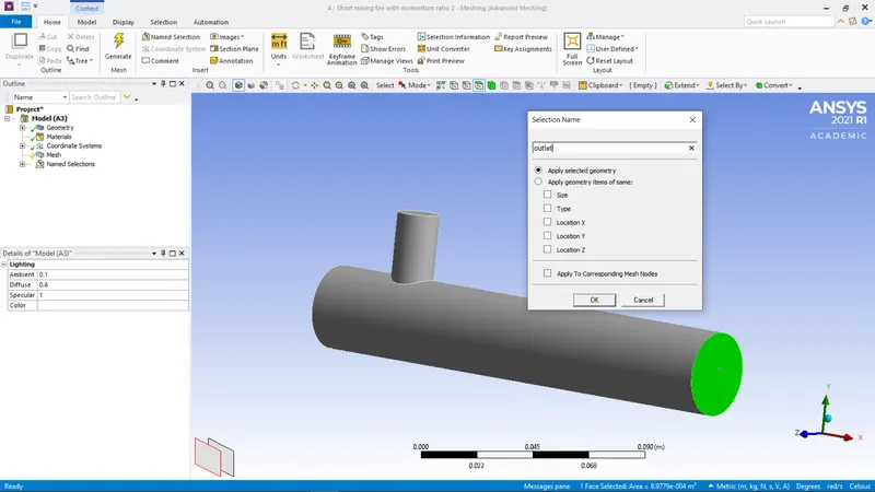
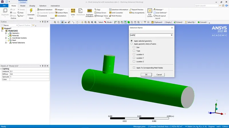
8. Now click on the mesh option then right click then choose to generate mesh here we are providing element size as 0.002. then go to quality ->mesh matric -> element quality. then close the mesh.

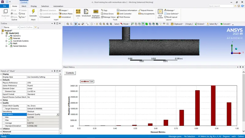
9. Double click setup, it will open fluent launcher then click double precision.

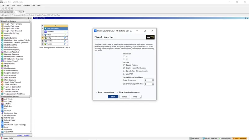
10. Ansys Fluent is opened. Graphics and console windows are displayed.

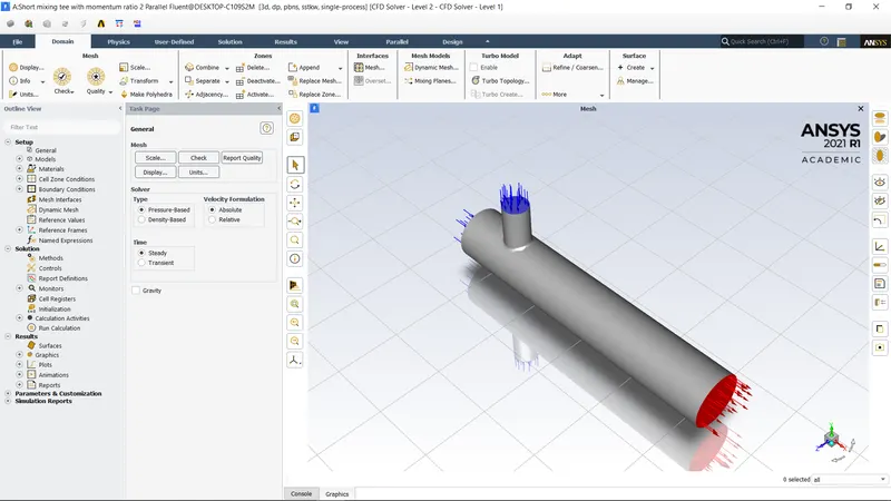
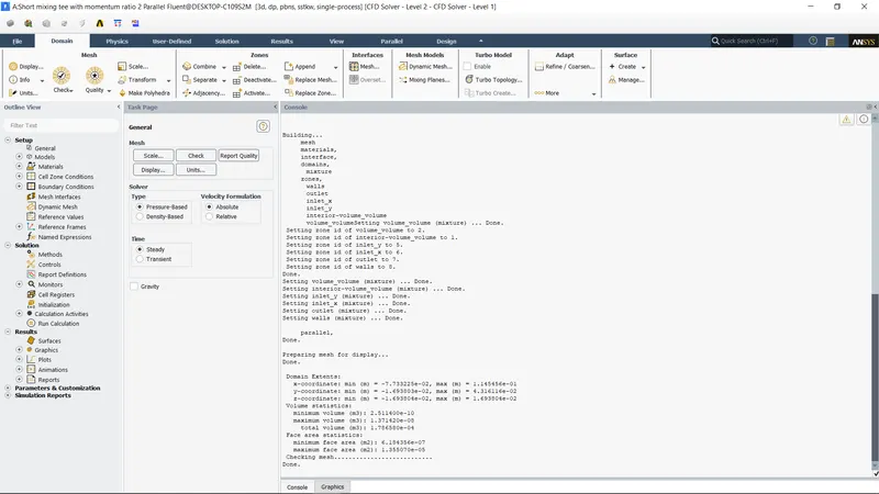
11. In the Domain -> Mesh -> select Check. In the console window, it shows checking mesh....done.

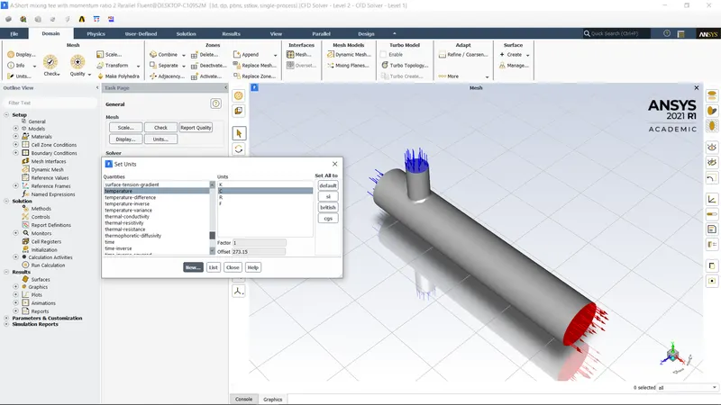
12. To change the units, click Units selected temperature and C then close.

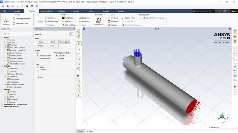
13. Setting up physics -> Solver -> select Time:Steady, Type:Pressure based, Velocity formation:Absolute.

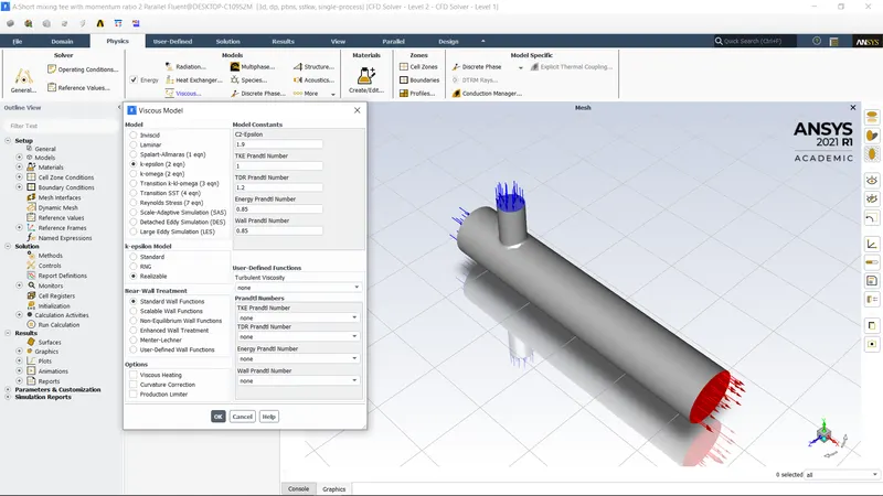
14. Setting up physics -> select Energy, select Viscous model -> K-epsilon model, Realizable K-epsilon model, standard wall functions -> Ok.

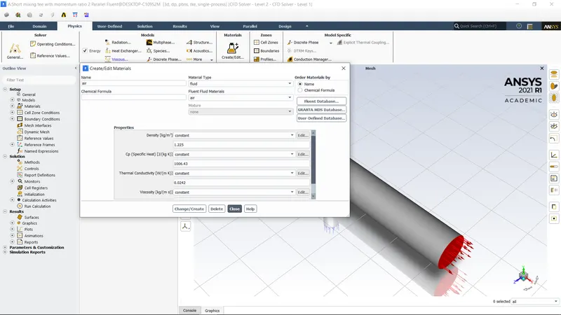
15. Click on material and choose air as working fluid.

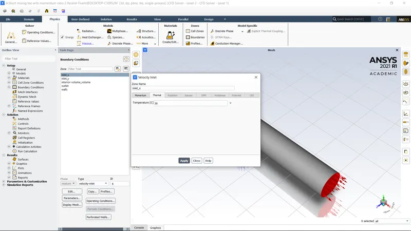
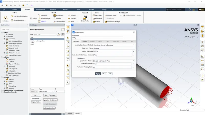
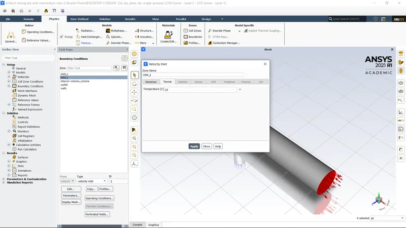
16. Setting up physics -> Boundaries -> Enter the values for momentum, thermal for both inlet x and inlet y. then click ok.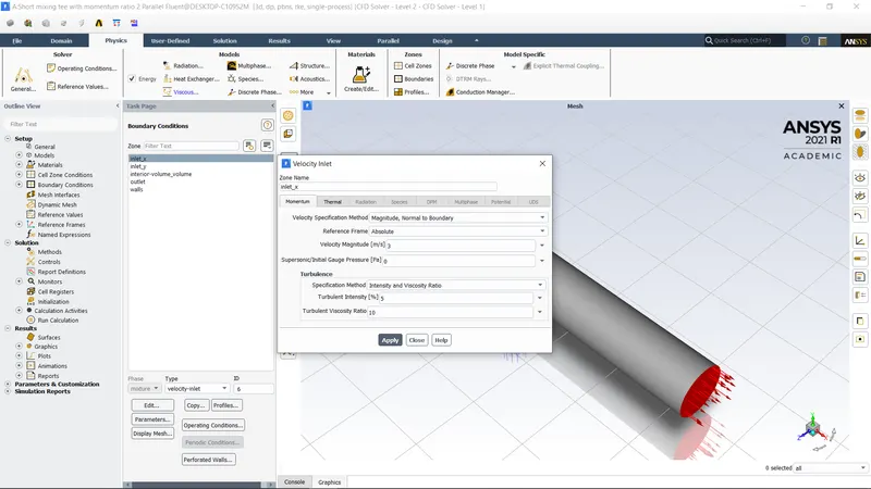

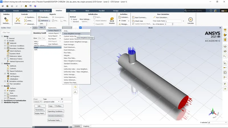
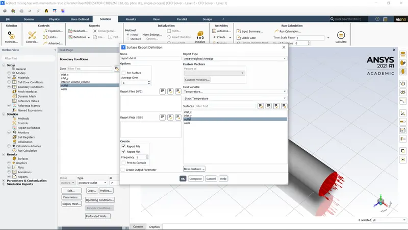
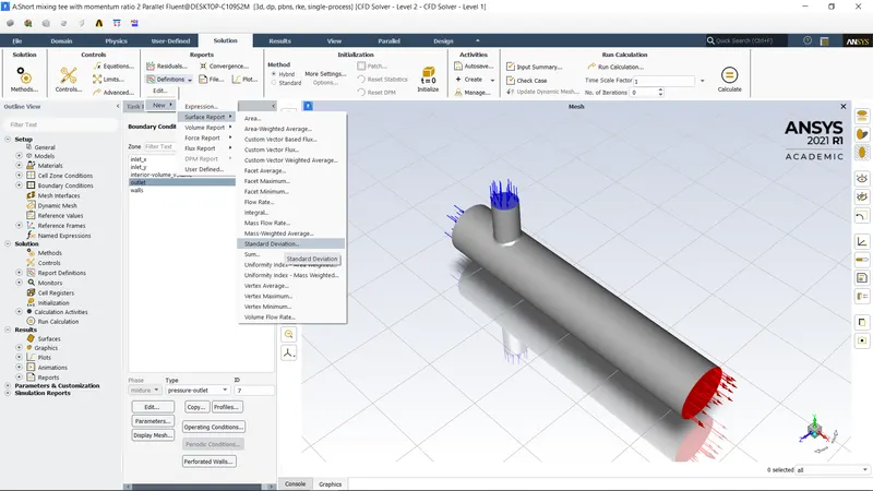
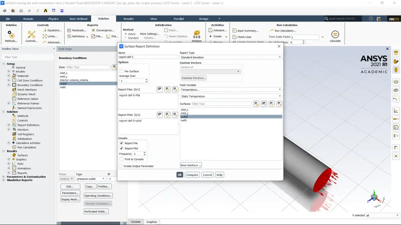
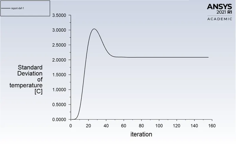
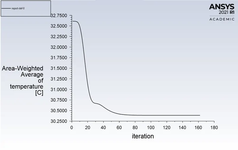
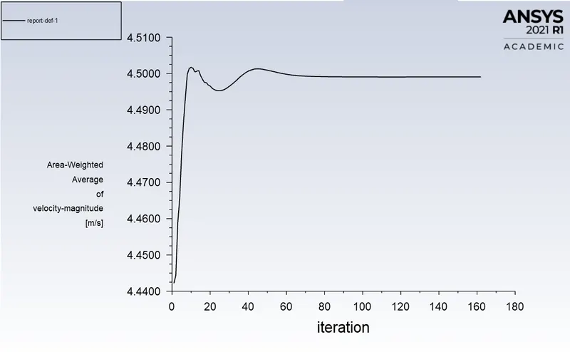
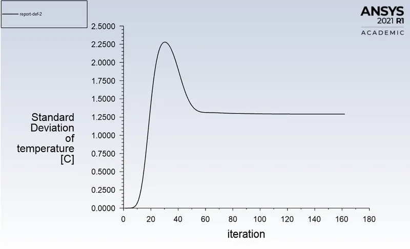
17. Go to Solution -> Reports -> Definitions -> New -> Surface Report -> Area weighted Average. similarly select Standard deviation. Then select the field variable -> Temperature. Create -> select Report File and Report Plot.

18. Initialization -> select method -> Hybrid -> click t=0 Initialize. then Run Calculation -> No. of iterations= 300 and press Calculate.

19. Exit setup and double click on the result to open the CFD post. Checkboxes to see walls and other parts. Click on walls and go to render set transparency of 0.9. color can also be changed to white for clear visibility.

20. Now insert planes, lines to plot the required plots for this project.

RESULTS:

Case 1:

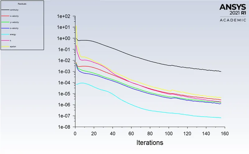
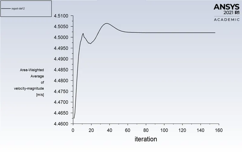
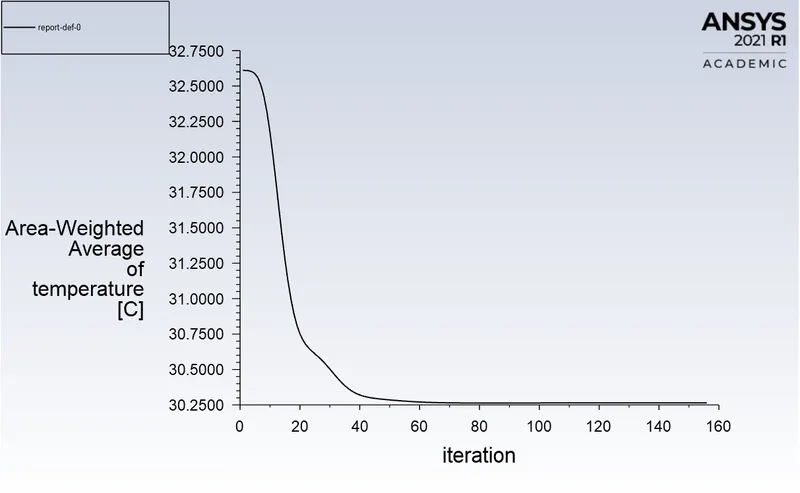
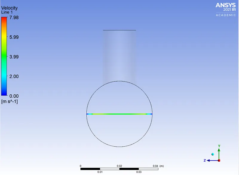
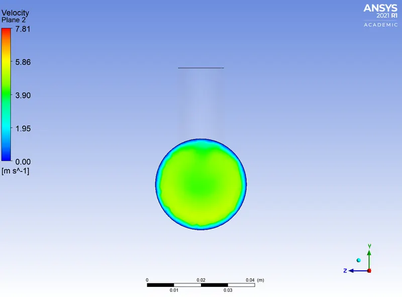
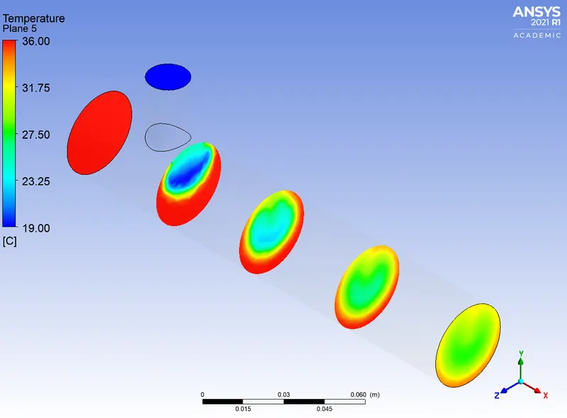
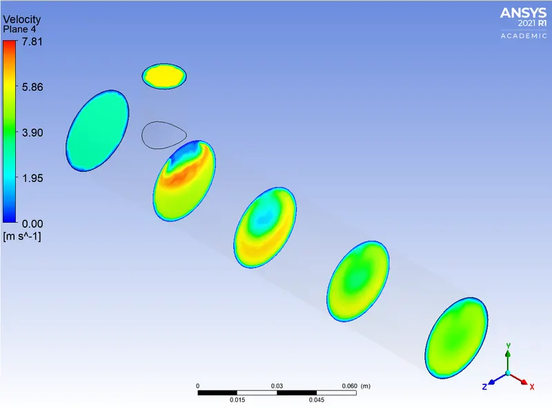
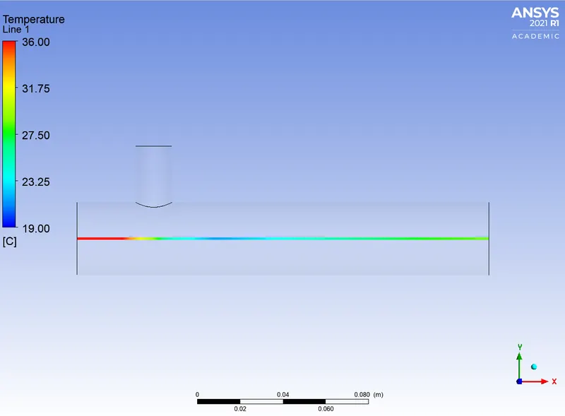
(a). Short mixing tee with a hot inlet velocity of 3 m/s, momentum ratio = 2 (Model used K-epsilon)

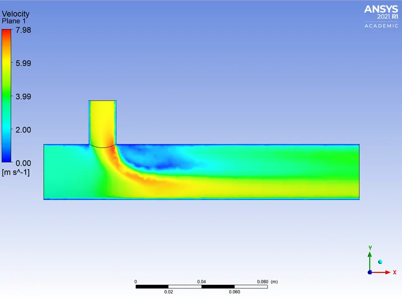
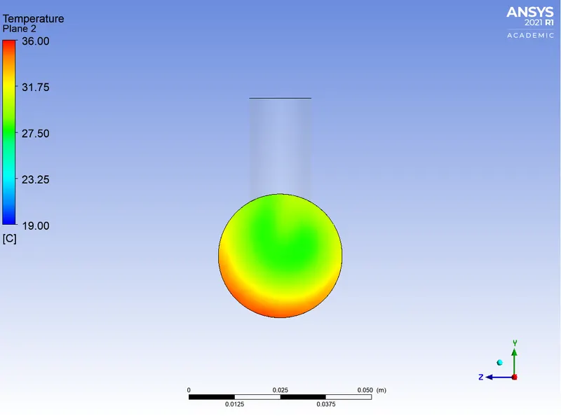
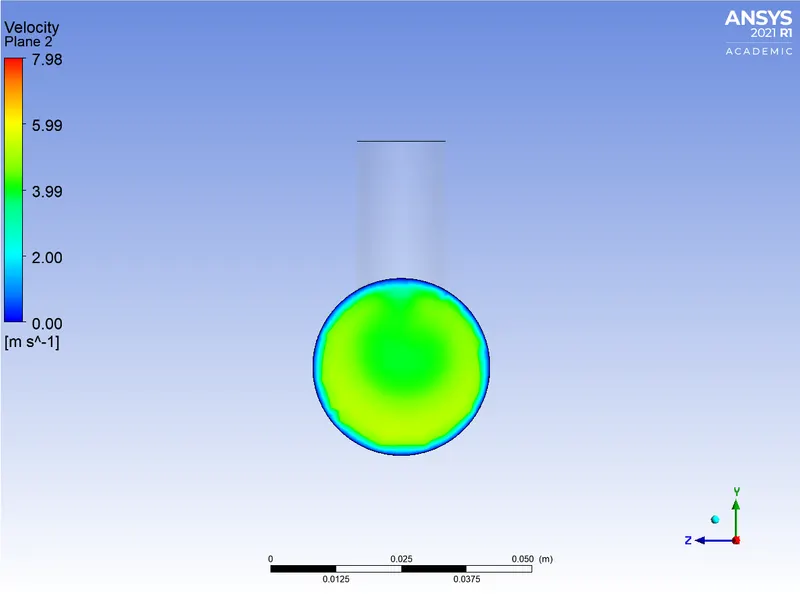
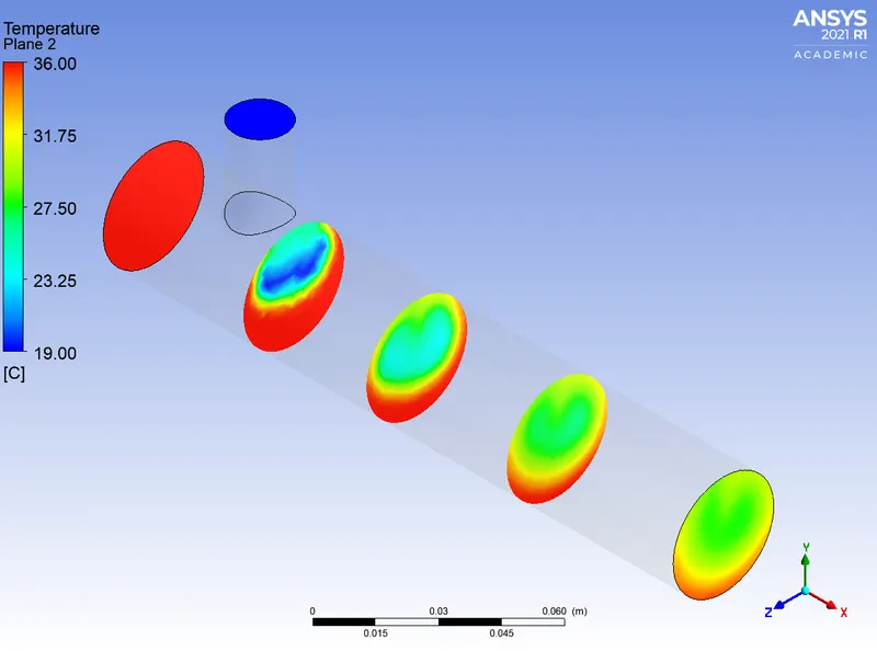
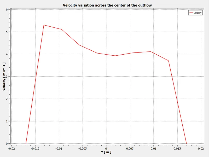
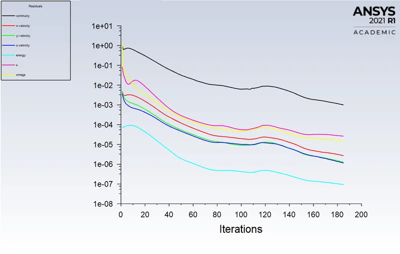
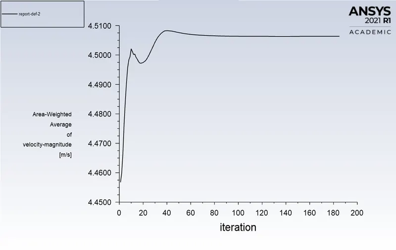
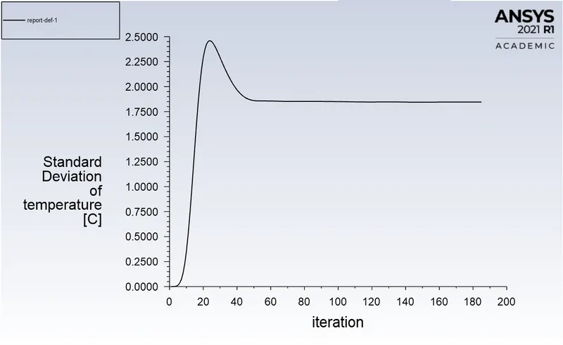
(b). Short mixing tee with a hot inlet velocity of 3 m/s, momentum ratio = 2 (Model used K-omega)

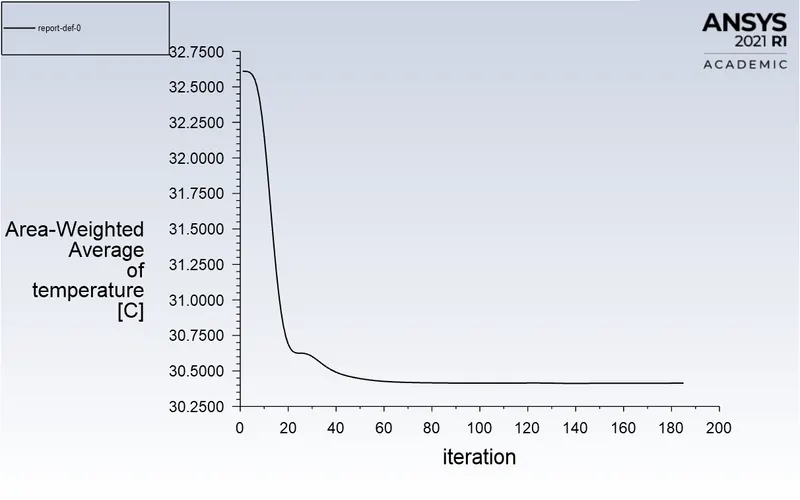
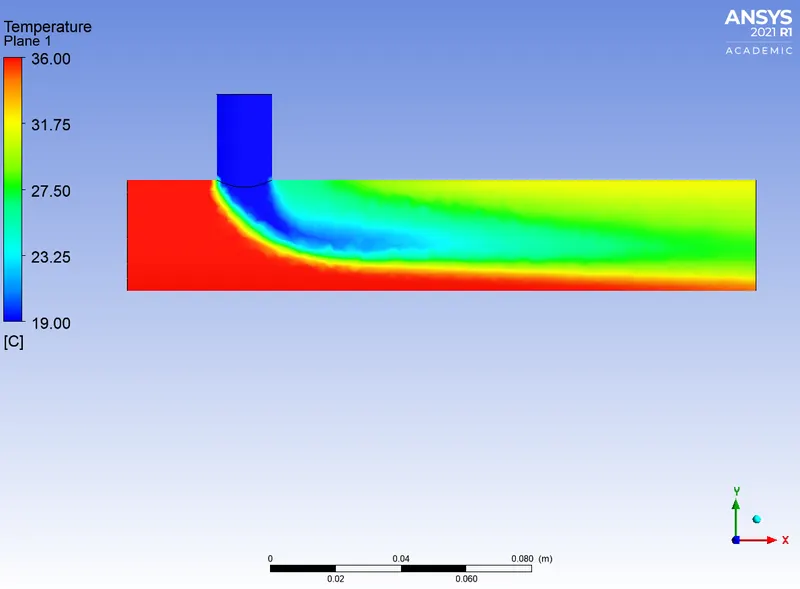
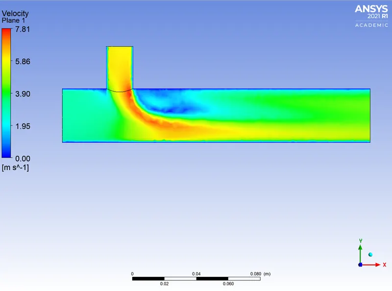
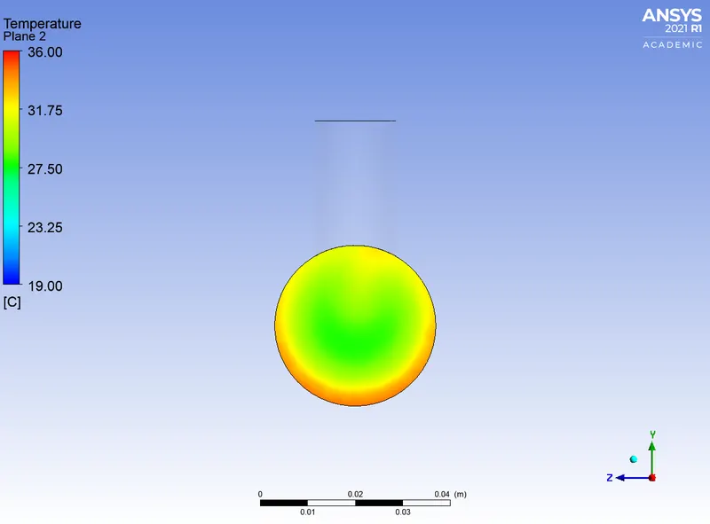
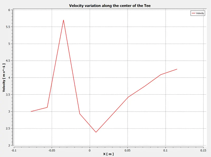
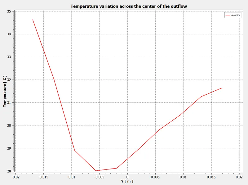
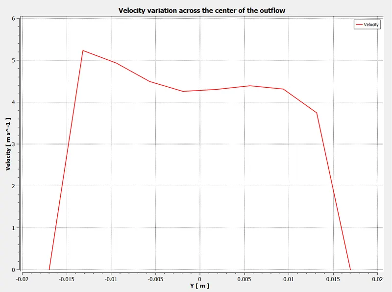
Summary:

K-epsilon K-omega

Cell count 105946 105946

Average Outlet Temperature 30.26503 C 30.41407 C

Number of iterations 156 185

Conclusion:

For momentum ratio 2, the K-epsilon model takes fewer iterations than the k-omega model. K-epsilon model takes less computation time to converge. Hence the K-epsilon model is faster to converge the solutions.

Therefore we can use the K-epsilon model for future calculations.

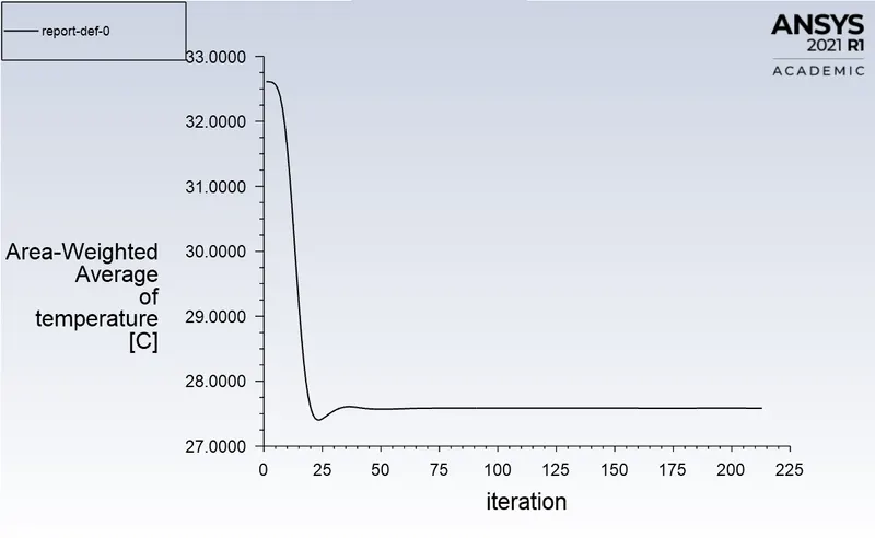
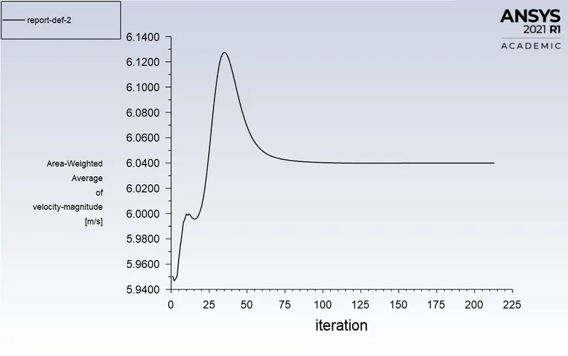
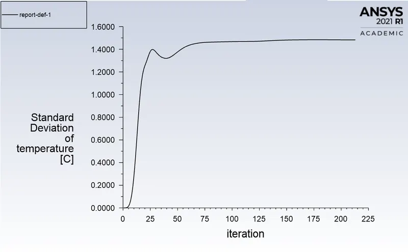
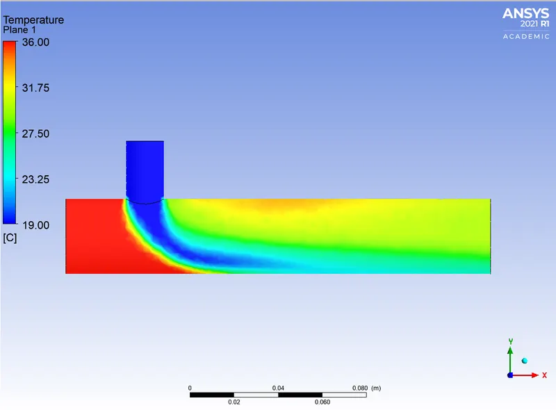
(c). Short mixing tee with a hot inlet velocity of 3 m/s, momentum ratio = 4 (Model used K-epsilon)

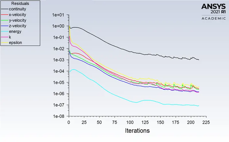
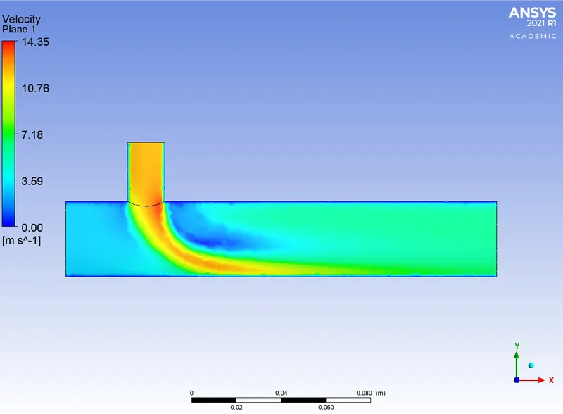
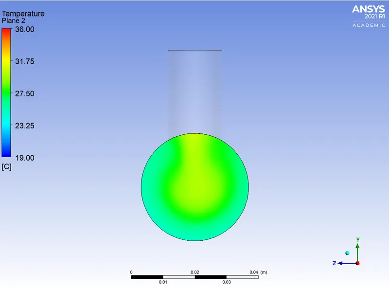
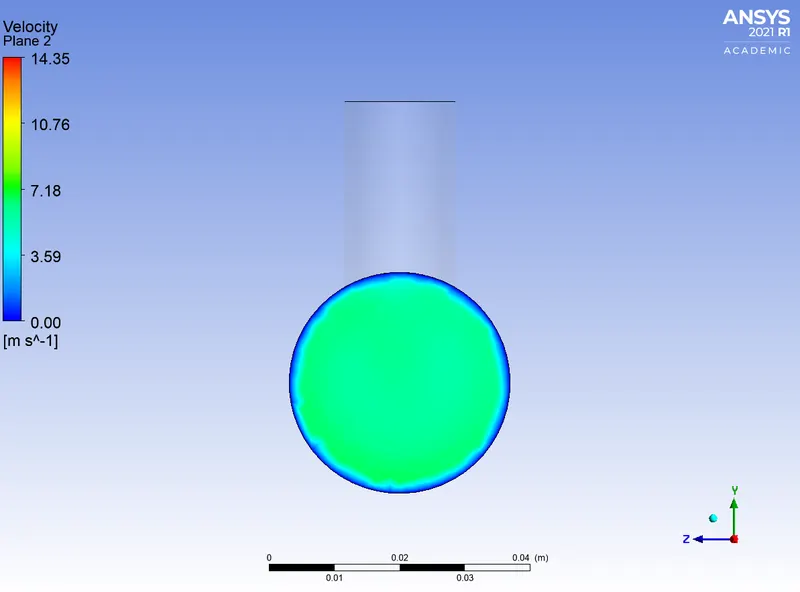
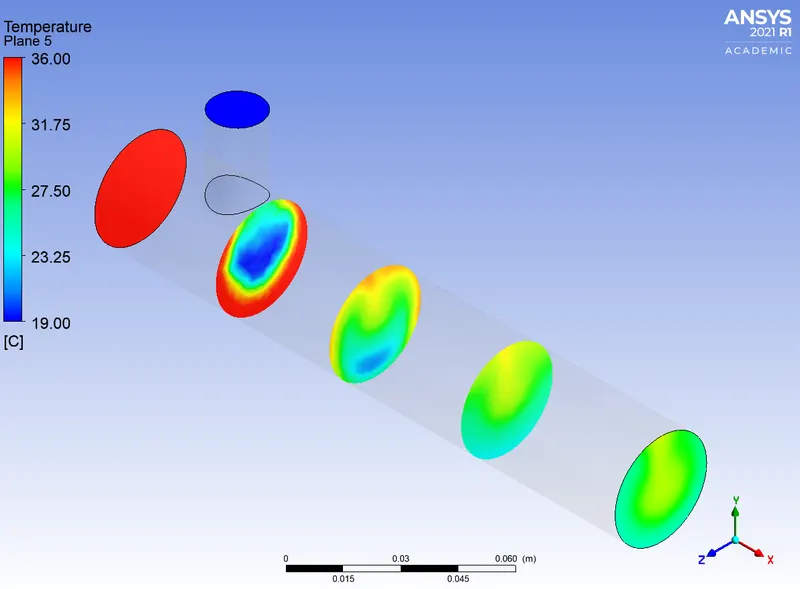
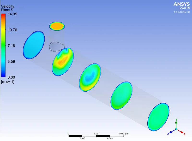
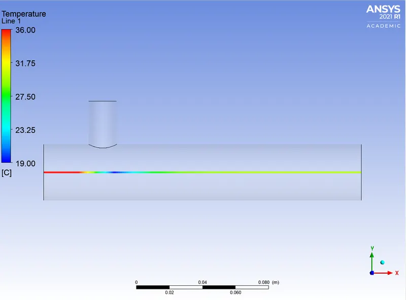
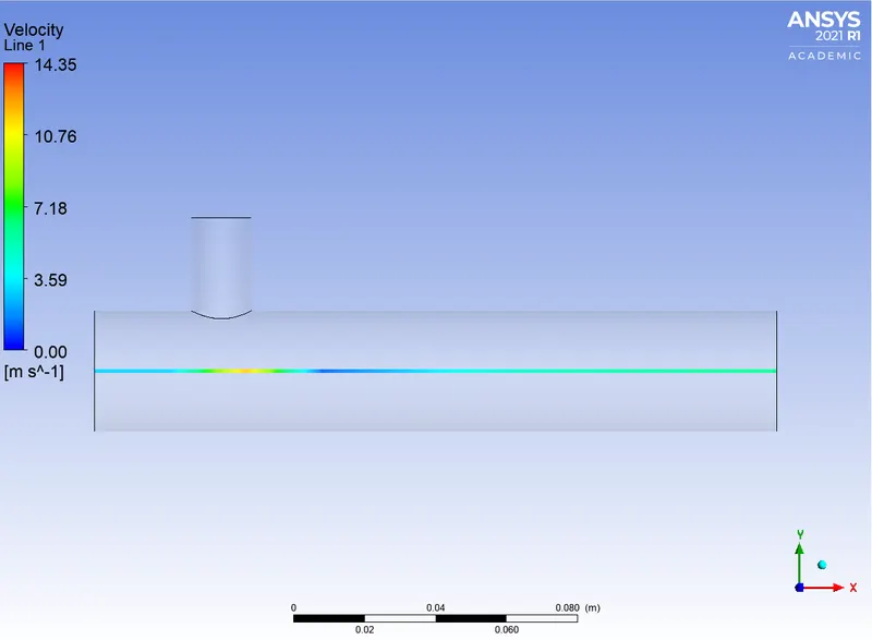
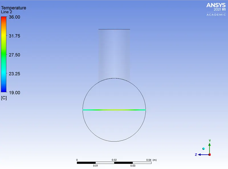
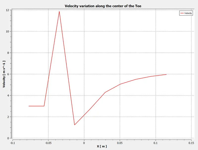
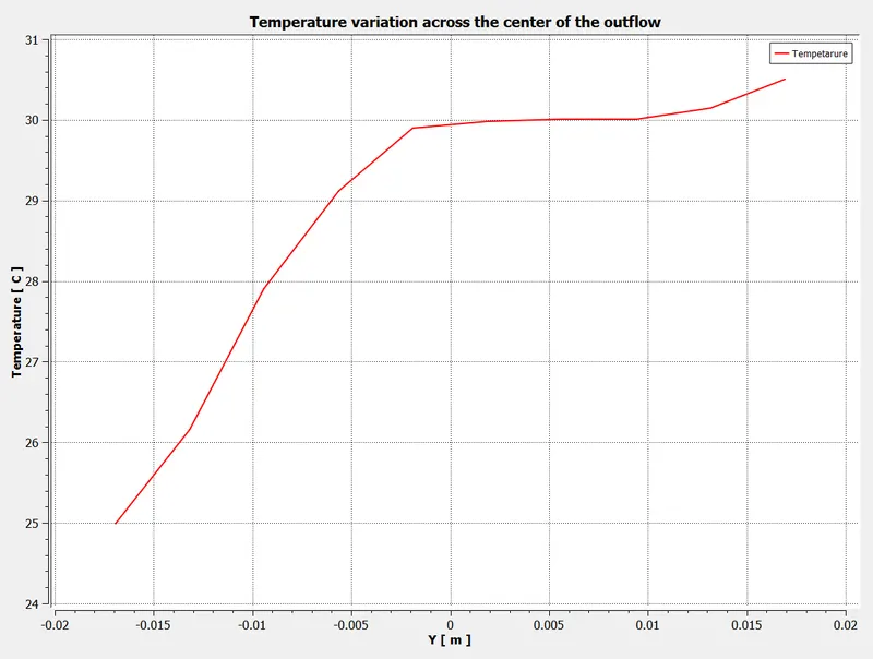
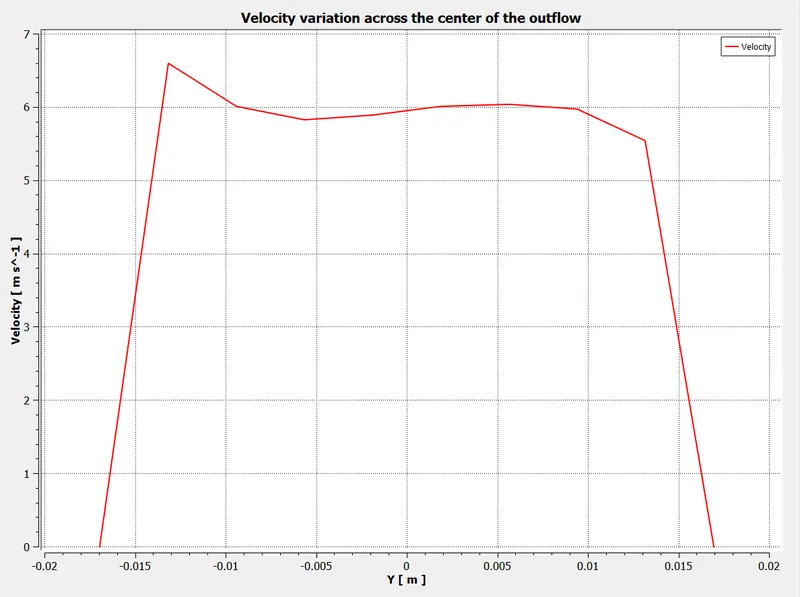
Case 2:

(a). Long mixing tee with a hot inlet velocity of 3 m/s, momentum ratio = 2 (Model used K-epsilon)

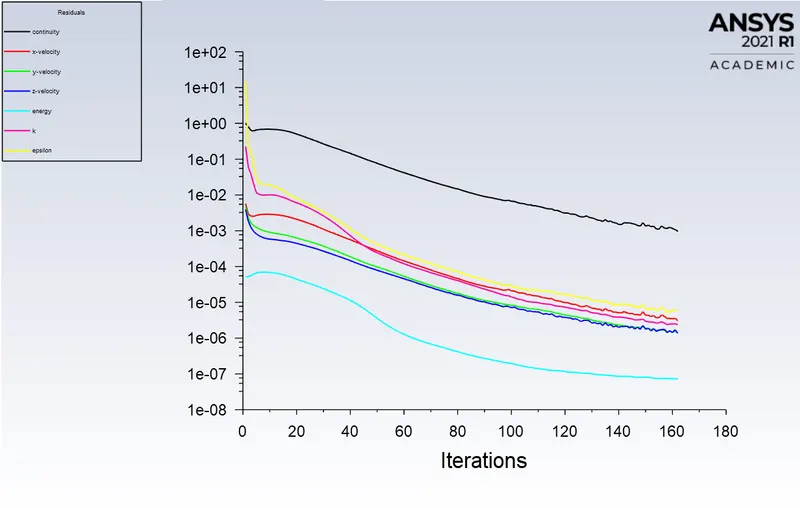
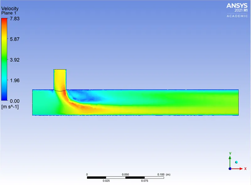
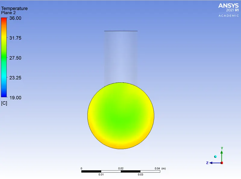
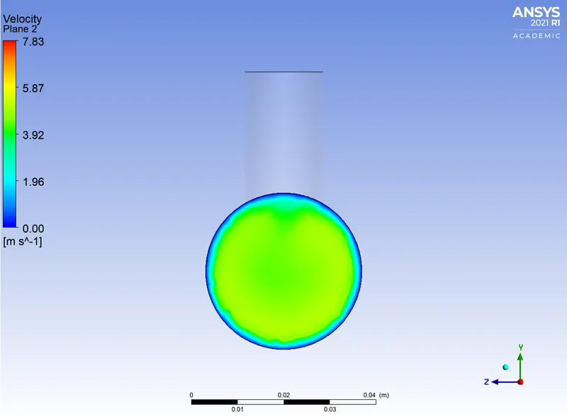
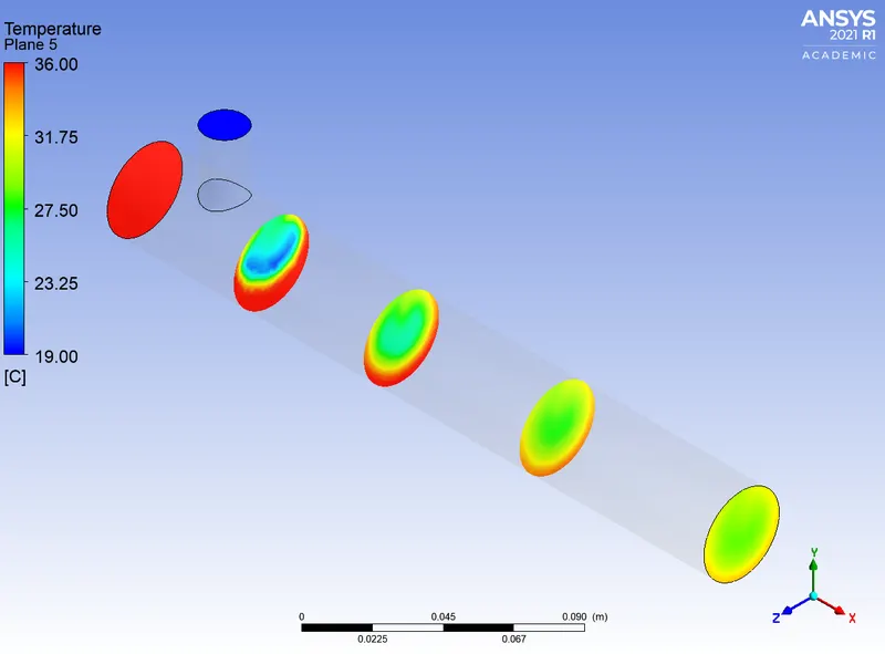
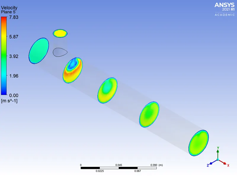
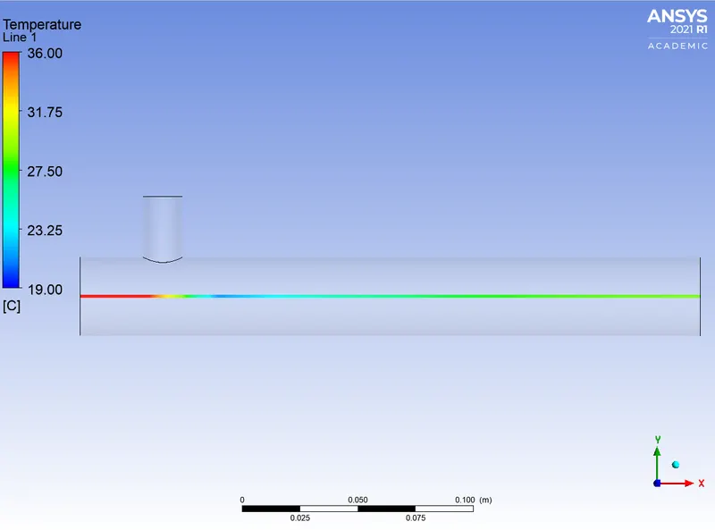
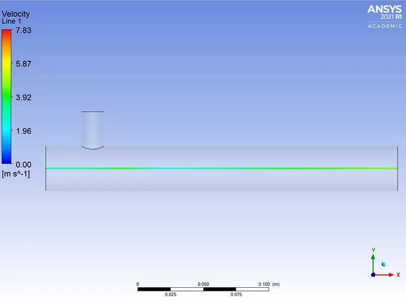
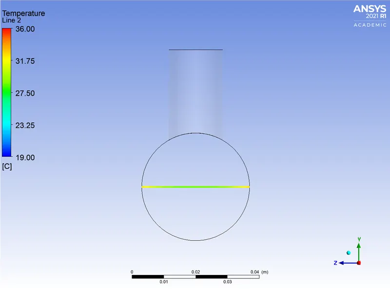
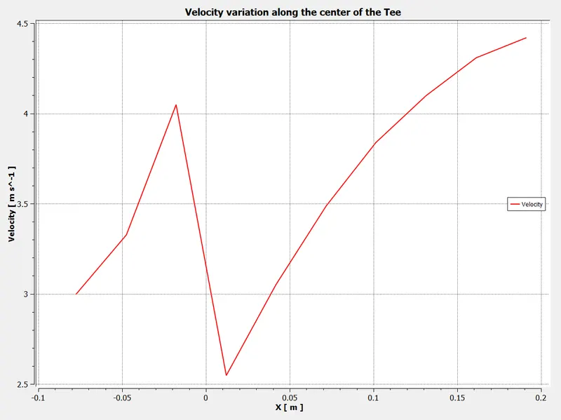
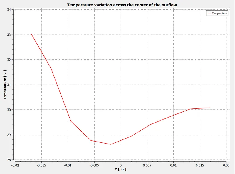
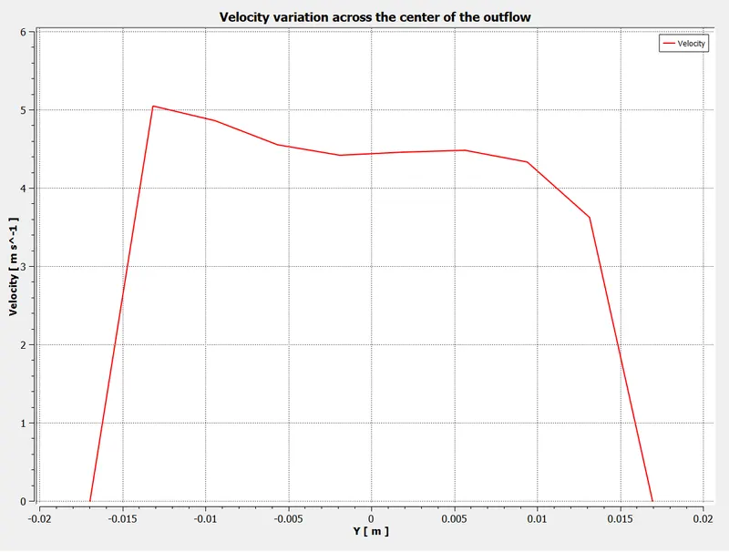
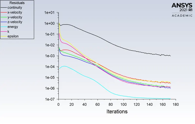
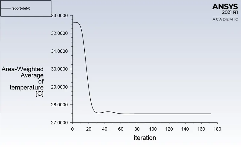
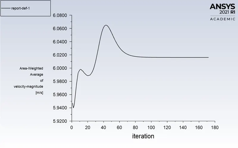
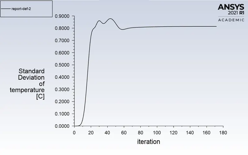
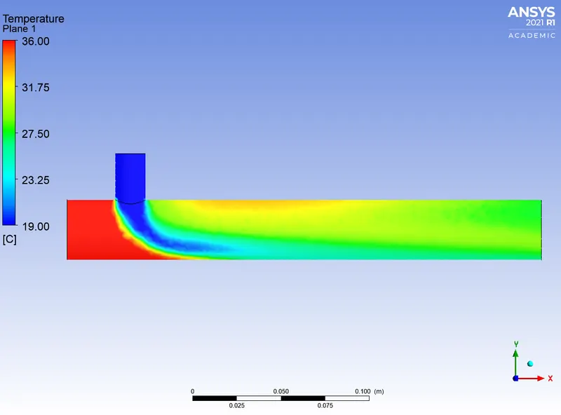
(b). Long mixing tee with a hot inlet velocity of 3 m/s, momentum ratio = 4 (Model used K-epsilon)

Summary:

Summary of comparison between Momentum ratio 2 and 4:

1. Short mixing tee:

a. (with K-epsilon)

Momentum Ratio 2 4

Cell counts 105946 105946

Number of iterations for the convergence 156 213

Outlet Temperature 30.26503 27.5861

b. (with K-omega)

Momentum Ratio 2

Cell counts 105946

Number of iterations for the convergence 185

Outlet Temperature 30.41407

2. Long mixing tee: (with K-epsilon)

Momentum Ratio 2 4

Cell counts 140025 140025

Number of iterations for the convergence 162 172

Outlet Temperature 30.38788 27.48958