Week 11 - Simulation of Flow through a pipe in OpenFoam
OBJECTIVE:
- Simulate the laminar flow through a pipe.
- To write the Matlab/Octave code dor blockMeshDict file.
- To post-process the results to validate fully developed flow velocity profile, to validate maximum velocity and pressure drop for fully developed flow, to validate shear stress for fully developed flow.
SOLUTION:
In this project, To understand various aspects of flow through a pipe, we are simulating in a section of pipe (wedge-shaped ). We are assuming the fluid is water and the flow is laminar and incompressible.
Fluid velocity in a pipe changes from zero at the surface, because of the no-slip condition, to a maximum at the pipe center. The average velocity remains constant in an incompressible flow when the cross-section of the pipe is constant.
Hydrodynamic entrance region and Hydrodynamically fully developed region:
The region from the pipe inlet to the point at which the velocity boundary layer merges at the centreline is called the hydrodynamic entrance region. The region beyond the entrance region in which the velocity profile is fully developed is called the hydrodynamically fully developed region.
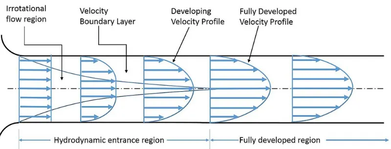
By definition, the entrance length for laminar flow through a pipe is defined in term of the Reynolds number as:
`L_(e) = 0.05R_(e)D`
Here we have to choose a diameter say 0.005 m
Then `L_(e) = 0.05 * 2100 * 0.005` `-> 0.525 m`
We have to assure that the length of the pipe is greater than the entrance length to simulate a fully developed flow.
So the length of the pipe is said `L = 1 m`
As here we are assuming that fluid is water and the fluid is at `25^0 C`. So properties of water at `25^0 C` is:
Density `rho = 997 (kg)/m^3`
Kinematic Viscosity `nu = 8.917*10^-7 m^2/s`
Dynamaic Viscosity `mu = nu*rho = 8.89*10^-4 (kg)/(ms)`
Applying Reynold's number formula:
`R_e = (v D)/nu`
where `v` is the velocity
Then `v = (R_e *nu)/D => (2100*8.917*10^-7)/(0.005) => 0.374514 m/s`
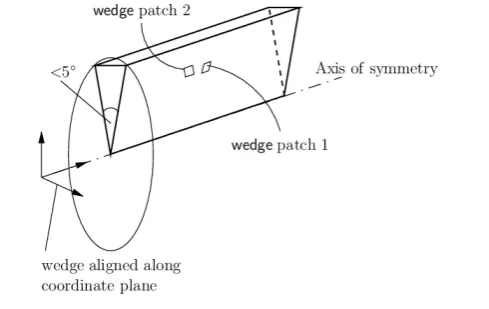
Now we know the geometric parameters of the pipe, we can reduce the model domain into a slice by choosing a value for the slice angle. Since the angle is very small, the curvature of the wall should not be that much different from a straight line.
BlockMeshDict File Auto-Generation Using Octave:
We will be utilizing the 'wedge' boundary condition available in OpenFOAM. The conditions in applying the wedge boundary are that the wedge angle should be less than `5^0`. For this project, we will be assessing the wedge angle of `4^0`.
The blockMeshDict file is generated using Octave so that we can easily change the wedge angle and generate another blockMeshDict file. The Octave code for generating the blockMeshDIct file and the file itself are attached below:
Octave Code:
clear all
close all
clc

L = 1;
theta = 4;
d = 0.005;
r = d/2;
nx = 500;
ny = 50;
nz = 1;


line1='/*---------------------------------*- C++ -*---------------------------------------*\';
line2='|  =========                 |                                                      |';
line3='|  \\      /  F ield         |  OpenFOAM: The Open Source CFD Toolbox               |';
line4='|   \\    /   O peration     |  Web:      https://openfoam.org                      |';
line5='|    \\  /    A nd           |  Version:  8                                         |';
line6='|     \\/     M anipulation  |                                                      |';
line7='\*---------------------------------------------------------------------------------*/';

line8='//*********************************************************************************//';

f1 = fopen('blockMesh.txt','w')
fprintf(f1,'%s\n',line1);
fprintf(f1,'%s\n',line2);
fprintf(f1,'%s\n',line3);
fprintf(f1,'%s\n',line4);
fprintf(f1,'%s\n',line5);
fprintf(f1,'%s\n',line6);
fprintf(f1,'%s\n',line7);


fprintf(f1,'FoamFile\n{\n');
fprintf(f1,'%12s \t 2.0;\n','version');
fprintf(f1,'%11s \t ascii;\n','format');
fprintf(f1,'%10s \t dictionary;\n','class');
fprintf(f1,'%11s \t blockMeshDict;\n','object');
fprintf(f1,'}\n');

fprintf(f1,'%s\n\n',line8);

fprintf(f1,'convertToMeters 1;\n\n');

fprintf(f1,'vertices\n');
fprintf(f1,'(\n');
fprintf(f1,'\t (%d %d %d)\n',0,0,0);                               % point 0
fprintf(f1,'\t (%d %d %d)\n',0,r*cosd(theta/2),r*sind(theta/2));   % point 1
fprintf(f1,'\t (%d %d %d)\n',0,r*cosd(theta/2),-r*sind(theta/2));  % point 2
fprintf(f1,'\t (%d %d %d)\n',L,0,0);                               % point 3
fprintf(f1,'\t (%d %d %d)\n',L,r*cosd(theta/2),r*sind(theta/2));   % point 4
fprintf(f1,'\t (%d %d %d)\n',L,r*cosd(theta/2),-r*sind(theta/2));  % point 5
fprintf(f1,');\n\n');

fprintf(f1,'blocks\n');
fprintf(f1,'(\n');
fprintf(f1,'\t hex (0 3 5 2 0 3 4 1) (%d %d %d)',nx,ny,nz);
fprintf(f1,' SimpleGrading (1 0.1 1)\n\n');
fprintf(f1,');\n\n');

fprintf(f1,'edges\n(\n\tarc %d %d (%d %d %d)\n',2,1,0,r,0);
fprintf(f1,'\tarc %d %d (%d %d %d)\n',5,4,L,r,0);
fprintf(f1,');\n\n');

fprintf(f1,'boundary\n(\n');
fprintf(f1,'\t inlet\n');
fprintf(f1,'\t{\n');
fprintf(f1,'\t\t type patch;\n');
fprintf(f1,'\t\t faces\n');
fprintf(f1,'\t\t (\n');
fprintf(f1,'\t\t\t (0 1 2 0)\n');
fprintf(f1,'\t\t );\n');
fprintf(f1,'\t}\n');

fprintf(f1,'\t outlet\n');
fprintf(f1,'\t{\n');
fprintf(f1,'\t\t type patch;\n');
fprintf(f1,'\t\t faces\n');
fprintf(f1,'\t\t (\n');
fprintf(f1,'\t\t\t (3 5 4 3)\n');
fprintf(f1,'\t\t );\n');
fprintf(f1,'\t}\n');

fprintf(f1,'\t top\n');
fprintf(f1,'\t{\n');
fprintf(f1,'\t\t type wall;\n');
fprintf(f1,'\t\t faces\n');
fprintf(f1,'\t\t (\n');
fprintf(f1,'\t\t\t (1 4 5 2)\n');
fprintf(f1,'\t\t );\n');
fprintf(f1,'\t}\n');

fprintf(f1,'\t back\n');
fprintf(f1,'\t{\n');
fprintf(f1,'\t\t type wedge;\n');
fprintf(f1,'\t\t faces\n');
fprintf(f1,'\t\t (\n');
fprintf(f1,'\t\t\t (0 2 5 3)\n');
fprintf(f1,'\t\t );\n');
fprintf(f1,'\t}\n');

fprintf(f1,'\t front\n');
fprintf(f1,'\t{\n');
fprintf(f1,'\t\t type wedge;\n');
fprintf(f1,'\t\t faces\n');
fprintf(f1,'\t\t (\n');
fprintf(f1,'\t\t\t (0 3 4 1)\n');
fprintf(f1,'\t\t );\n');
fprintf(f1,'\t}\n');

fprintf(f1,'\t axis\n');
fprintf(f1,'\t{\n');
fprintf(f1,'\t\t type empty;\n');
fprintf(f1,'\t\t faces\n');
fprintf(f1,'\t\t (\n');
fprintf(f1,'\t\t\t (0 3 3 0)\n');
fprintf(f1,'\t\t );\n');
fprintf(f1,'\t}\n');
fprintf(f1,');\n\n');

fprintf(f1,'mergePatchPairs\n(\n');
fprintf(f1,');\n');

fprintf(f1,'%s\n',line8);

fclose(f1)
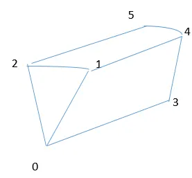
Providing vertices according to the above sketch
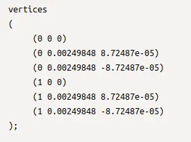
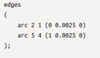
Each edge joining 2 vertex points is assumed to be straight by default. However, any edge may be specified to be curved by entries. Each entry for a curved edge begins with a keyword specifying the type of the curve.
The keyword is then followed by the labels of the 2 vertices that the edge connects. Following that, interpolation points must be specified through which the edge passes. For an arc, a single interpolation point is required, which the circular arc will intersect.
In our case, we are specifying arc edge connecting vertices 2 and 1, 5 and 4.
blockMeshDict File:
/*---------------------------------*- C++ -*---------------------------------------*\
|  =========                 |                                                      |
|  \\      /  F ield         |  OpenFOAM: The Open Source CFD Toolbox               |
|   \\    /   O peration     |  Web:      https://openfoam.org                      |
|    \\  /    A nd           |  Version:  8                                         |
|     \\/     M anipulation  |                                                      |
\*---------------------------------------------------------------------------------*/
FoamFile
{
     version 	 2.0;
     format 	 ascii;
     class 	 dictionary;
     object 	 blockMeshDict;
}
//*********************************************************************************//

convertToMeters 1;

vertices
(
	 (0 0 0)
	 (0 0.00249848 8.72487e-05)
	 (0 0.00249848 -8.72487e-05)
	 (1 0 0)
	 (1 0.00249848 8.72487e-05)
	 (1 0.00249848 -8.72487e-05)
);

blocks
(
	 hex (0 3 5 2 0 3 4 1) (500 50 1) SimpleGrading (1 0.1 1)

);

edges
(
	arc 2 1 (0 0.0025 0)
	arc 5 4 (1 0.0025 0)
);

boundary
(
	 inlet
	{
		 type patch;
		 faces
		 (
			 (0 1 2 0)
		 );
	}
	 outlet
	{
		 type patch;
		 faces
		 (
			 (3 5 4 3)
		 );
	}
	 top
	{
		 type wall;
		 faces
		 (
			 (1 4 5 2)
		 );
	}
	 back
	{
		 type wedge;
		 faces
		 (
			 (0 2 5 3)
		 );
	}
	 front
	{
		 type wedge;
		 faces
		 (
			 (0 3 4 1)
		 );
	}
	 axis
	{
		 type empty;
		 faces
		 (
			 (0 3 3 0)
		 );
	}
);

mergePatchPairs
(
);
//*********************************************************************************//
Initial and Boundary Conditions:
Pressure:
/*--------------------------------*- C++ -*----------------------------------*\
  =========                 |
  \\      /  F ield         | OpenFOAM: The Open Source CFD Toolbox
   \\    /   O peration     | Website:  https://openfoam.org
    \\  /    A nd           | Version:  8
     \\/     M anipulation  |
\*---------------------------------------------------------------------------*/
FoamFile
{
    version     2.0;
    format      ascii;
    class       volScalarField;
    object      p;
}
// * * * * * * * * * * * * * * * * * * * * * * * * * * * * * * * * * * * * * //

dimensions      [0 2 -2 0 0 0 0];

internalField   uniform 0;

boundaryField
{
    inlet
    {
        type            zeroGradient;
    }

    outlet
    {
        type            fixedValue;
        value           uniform 0;
    }

    axis
    {
        type            empty;
    }

    top
    {
        type            zeroGradient;
    }

    front
    {
        type            wedge;
    }

    back
    {
        type            wedge;
    }
}

// ************************************************************************* //
Velocity:
/*--------------------------------*- C++ -*----------------------------------*\
  =========                 |
  \\      /  F ield         | OpenFOAM: The Open Source CFD Toolbox
   \\    /   O peration     | Website:  https://openfoam.org
    \\  /    A nd           | Version:  8
     \\/     M anipulation  |
\*---------------------------------------------------------------------------*/
FoamFile
{
    version     2.0;
    format      ascii;
    class       volVectorField;
    object      U;
}
// * * * * * * * * * * * * * * * * * * * * * * * * * * * * * * * * * * * * * //

dimensions      [0 1 -1 0 0 0 0];

internalField   uniform (0 0 0);

boundaryField
{
    inlet
    {
        type            fixedValue;
        value           uniform (0.374514 0 0);
    }

    outlet
    {
        type            zeroGradient;
    }

    axis
    {
        type            empty;
    }

    top
    {
        type            noSlip;
    }

    front
    {
        type            wedge;
    }

    back
    {
        type            wedge;
    }
}

// ************************************************************************* //
`CFL = U(Deltat)/(Deltax) <=1`
where `Deltax =` (Length of the pipe)/(number of cell in x direction)
`Deltax = 1/500 = 0.002`
U = 0.374514 m/s
`Deltat <= (Deltax)/U => Deltat<=0.002/0.374514 =>Deltat<= 0.005`
To control max courant number we can consider delta t = 0.0005 s
The simulation is run for a total time of 5 second.
ControlDict File:
/*--------------------------------*- C++ -*----------------------------------*\
  =========                 |
  \\      /  F ield         | OpenFOAM: The Open Source CFD Toolbox
   \\    /   O peration     | Website:  https://openfoam.org
    \\  /    A nd           | Version:  8
     \\/     M anipulation  |
\*---------------------------------------------------------------------------*/
FoamFile
{
    version     2.0;
    format      ascii;
    class       dictionary;
    location    "system";
    object      controlDict;
}
// * * * * * * * * * * * * * * * * * * * * * * * * * * * * * * * * * * * * * //

application     icoFoam;

startFrom       startTime;

startTime       0;

stopAt          endTime;

endTime         5;

deltaT          0.0005;

writeControl    timeStep;

writeInterval   20;

purgeWrite      0;

writeFormat     ascii;

writePrecision  6;

writeCompression off;

timeFormat      general;

timePrecision   6;

runTimeModifiable true;


// ************************************************************************* //
Transport Properties:
/*--------------------------------*- C++ -*----------------------------------*\
  =========                 |
  \\      /  F ield         | OpenFOAM: The Open Source CFD Toolbox
   \\    /   O peration     | Website:  https://openfoam.org
    \\  /    A nd           | Version:  8
     \\/     M anipulation  |
\*---------------------------------------------------------------------------*/
FoamFile
{
    version     2.0;
    format      ascii;
    class       dictionary;
    location    "constant";
    object      transportProperties;
}
// * * * * * * * * * * * * * * * * * * * * * * * * * * * * * * * * * * * * * //

nu              [0 2 -1 0 0 0 0] 8.917e-7;


// ************************************************************************* //
Results:
Inlet: We can see the developing flow at the inlet of the pipe.
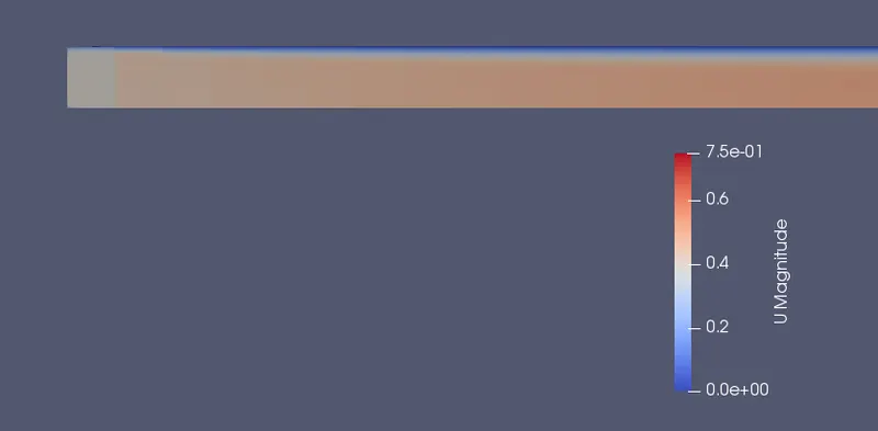
Outlet: We can see fully developed flow at the outlet of the pipe.
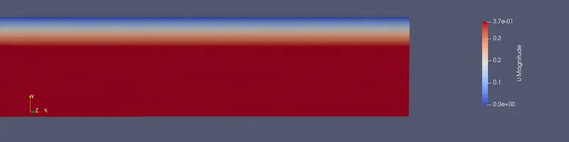
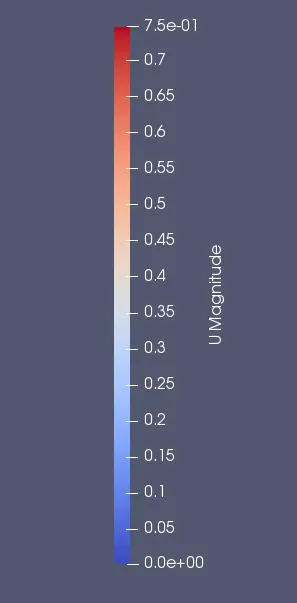
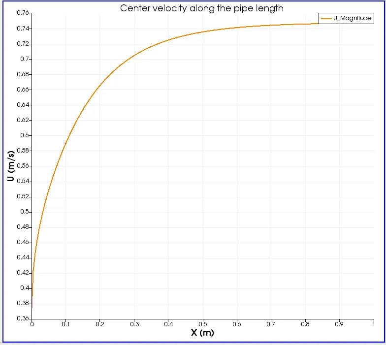
We can see that the flow is developed at a length of about 0.5m. the length of the entrance region which we have calculated is 0.525m.
Output Graphs:
Velocity distribution along the pipe length:
Pressure drop along the length of the pipe:
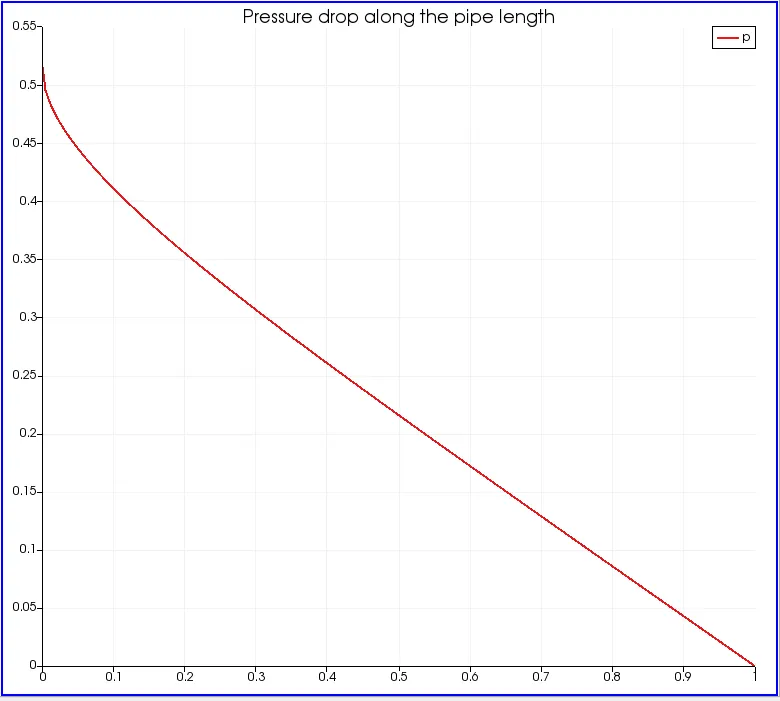
According to the Hagen-Poiseuile equation,
`Delta P = (32muLv)/(D^2)`
`DeltaP = (32*8.89*10^-4*1*0.374514)/(0.005^2) = 426.1669 (kg)/(m*s^2)`
Kinematic Pressure `P/rho`
KInematic pressure drop `(DeltaP)/rho = 426.1669/997 = 0.4274 m^2/s^2`
Velocity profiles at different lengths along the center of pipe from inlet:
The Reflect option is used to plot.
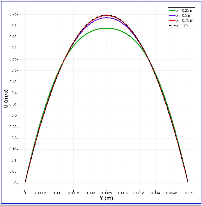
It is observed that the velocity profile gradually increased from the inlet to the outlet. we can see the maximum velocity at the outlet of the pipe.
This region is called a fully developed region. we can see velocity profile is completely developed at the outlet. The developing flow can be clearly seen from x = 0.25 to x = 0.5 m. and further along the length of the pipe.
The maximum velocity along the centerline for fully developed is, 2 times inlet velocity,
`U_(max) = 2*U = 2*0.374514 = 0.749028 m/s.`
The maximum velocity and pressure drop are compared with the results obtained from the numerical simulation
| Analytical Result | Result from Simulation | |
| Maximum Velocity | 0.74903 | 0.74705 |
| Pressure Drop | 0.4274 | 0.5139 |
Shear stress variation from outer walls to the center of the pipe:
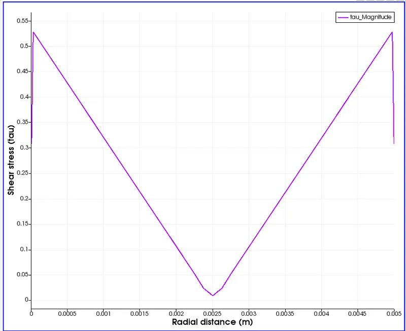
This plot shows the variation of shear stress across the radius of the pipe. The shear stress is maximum at the wall and zeroes at the pipe axis.
This plot is generated in Paraview. Firstly the magnitude of velocity is calculated with the calculator in the toolbar. Then gradient of the velocity is calculated using the gradients of the unstructured data set filter from the filter search option. then used the calculator to calculate the shear stress using the formula `tau = mu*((du)/(dx))`.
Then used the plot over line command to create a plot of shear stress.