Challenge

Week 12 - Validation studies of Symmetry BC vs Wedge BC in OpenFOAM vs Analytical H.P equation

VVikas Rai16 Jun 2021

OBJECTIVE:

To write a program in Matlab/Octave to create a blockMeshDict file for different `theta` values. for two boundary conditions wedge boundary condition and symmetry boundary condition. Angle to be tested are 10, 25, and 45 degrees.
The other objective is to post-process the velocity results at different length of the pipe and shear stress at the fully developed region and compare it with the analytical solution, i.e. by the Hagen poiseuille equation and wedge boundary conditions.
The final objective is to validate the fully developed flow velocity profile with its analytical profile, validate maximum velocity and pressure drop for fully developed flow, and highlight the differences in both boundary conditions.

INTRODUCTION:

Liquid or gas flow through pipes or ducts is commonly used in heating and cooling applications and fluid distribution networks. The fluid in such applications is usually forced to flow by a fan or pump through a flow section. We pay particular attention to friction, which is directly related to the pressure drop and head loss during flow through pipes and ducts. The pressure drop is then used to determine the pumping power requirement. A typical piping system involves pipes of different diameters connected to each other by various fittings or elbows to route the fluid, valves to control the flow rate, and pumps to pressurize the fluid.

The fluid velocity in a pipe changes from zero at the wall because of the no-slip condition to a maximum at the pipe center. In fluid flow, it is convenient to work with an average velocity `V_(avg)`, which remains constant in incompressible flow when the cross-sectional area of the pipe is constant. The average velocity in heating and cooling applications may change somewhat because of changes in density with temperature. But, in practice, we evaluate the fluid properties at some average temperature and treat them as constants.

Laminar Flow:

Laminar or streamline flow in pipes or tubes occurs when a fluid flows in parallel layers, with no disruption between the layers. At low velocities, the fluid tends to flow without lateral mixing, and adjacent layers slide one another. There are no cross-currents perpendicular to the direction of flow, no swirls of fluids. In laminar flow, the motion of the particles of the fluid is very orderly with all particles moving in straight lines parallel to the pipe walls.

Turbulent Flow:

Turbulent flow is a flow regime characterized by chaotic property changes. This includes a rapid variation of pressure and flows velocity in space and time. Turbulent flow is a type of fluid flow in which the fluid undergoes irregular fluctuations, or mixing in contrast to laminar flow, in which the fluid moves in smooth paths or layers. In turbulent flow, the speed of the fluid at a point is continuously undergoing changes in both magnitude and direction.

Reynolds Number:

The Reynolds number is the ratio of inertial forces to viscous forces within a fluid. This is expressed for internal flow in a circular pipe as

`Re = (In ertial fo rces )/ (Viscous fo rces ) = (V_(avg) D )/nu = (rho V_(avg)D)/mu`

where `V_(avg)` = average flow velocity (m/s)

D = diameter of pipe (m)

`nu = mu/rho =` kinematic viscosity of the fluid (`m^2/s`)

Note that the Reynolds number is a dimensionless quantity. The Reynolds number (Re) helps predict flow patterns in different fluid flow situations. At low Reynolds numbers, flows tend to be laminar flow, while at high Reynolds number flows tend to be turbulent.

The Reynolds number at which the flow becomes turbulent is called the critical Reynolds number, `Re_(cr)`. The value of the critical Reynolds number is different geometries and flow conditions. For internal flow in a circular pipe, the generally accepted value of the critical Reynolds number is `Re_(cr) = 2300`.

Under most practical conditions, the flow in a circular pipe is:

`Re <= 2300` Laminar flow

`2300<= Re <= 4000` Transitional flow

`Re >= 4000` Turbulent flow

Hydrodynamic entrance region and Hydrodynamically fully developed region:

The region of the flow in which the effects of the viscous shearing forces caused by fluid viscosity are felt is called the velocity boundary layer or just the boundary layer. The hypothetical boundary surface divides the flow in a pipe into two regions: the boundary layer region, in which the viscous effects and the velocity changes are significant, and the irrotational flow region, in which the frictional effects are negligible and the velocity remains essentially constant in the radial direction.

The thickness of this boundary layer increases in the flow direction until the boundary layer reaches the pipe center and thus fills the entire pipe and the velocity becomes fully developed. The region from the pipe inlet to the point at which the velocity profile is fully developed is called the hydrodynamic entrance region, and the length of this region is called the hydrodynamic entry length `L_h`. Flow in the entrance region is called hydrodynamically developing flow since this is the region where the velocity profile develops. The region beyond the entrance region in which the velocity profile is fully developed and remains unchanged is called the hydrodynamically fully developed region.

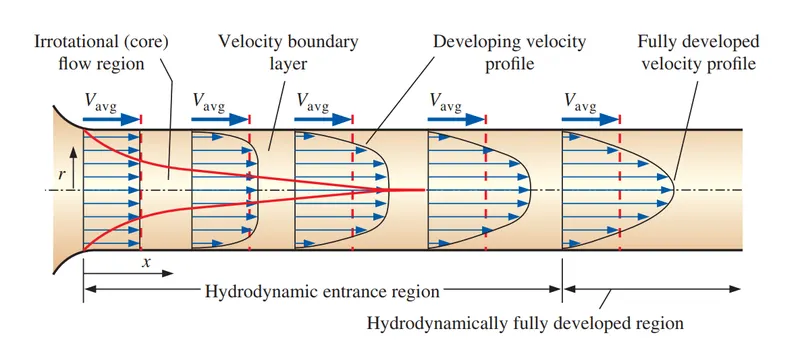
By definition, the entrance length for laminar flow through a pipe is defined in term of the Reynolds number as:

`L_(e) = 0.05R_(e)D`

Here we have to choose a diameter say 0.005 m

Then `L_(e) = 0.05 * 2100 * 0.005` `-> 0.525 m`

We have to assure that the length of the pipe is greater than the entrance length to simulate a fully developed flow.

So the length of the pipe is said `L = 1 m`

As here we are assuming that fluid is water and the fluid is at `25^0 C`. So properties of water at `25^0 C` is:

Density `rho = 997 (kg)/m^3`

Kinematic Viscosity `nu = 8.917*10^-7 m^2/s`

Dynamaic Viscosity `mu = nu*rho = 8.89*10^-4 (kg)/(ms)`

Applying Reynold's number formula:

`R_e = (v D)/nu`

where `v` is the velocity

Then `v = (R_e *nu)/D => (2100*8.917*10^-7)/(0.005) => 0.374514 m/s`

Now we know the geometric parameters of the pipe, we can reduce the model domain into a slice by choosing a value for the slice angle. The side walls need to be assigned some specific boundary conditions. The sides can be assigned a wedge or symmetry boundary condition.

Wedge boundary condition:

Wedge boundary conditions can be applied to very small angles (`<5^o`) not more than that. The wedge boundary condition also requires a single cell between the boundary pairs. But if any complexity in an axisymmetric boundary requires the angle to be more than 5 degrees, then the wedge boundary condition can not be used. This happens when a particular obstacle present which is not symmetric about the axis but to capture it in the geometry, the angle needs to be more than 5 degrees. This is the limitation for wedge boundary conditions.

Symmetry boundary condition:

Symmetry boundary conditions can be applied to larger angles. The symmetry boundary condition can discretize in multiple cells. This gives a slight advantage to the symmetry boundary condition, with this a more accurate circular surface can be generated rather than a straight line between the two wedge planes. No angular limit between the two symmetry planes in axisymmetric problems as in the wedge case.

BlockMeshDict File Auto-Generation Using Octave:

CASE 1: WEDGE BOUNDARY CONDITIONS

We will be utilizing the 'wedge' boundary condition available in OpenFOAM.

The blockMeshDict file is generated using Octave so that we can easily change the wedge angle and generate another blockMeshDict file. The Octave code for generating the blockMeshDIct files and the files themselves are attached below:

Octave Code:

clear all
close all
clc

% length of pipe
L = 1;

%wedge angle
theta = 4;

%Diameter of pipe
d = 0.005;
% Radius of pipe
r = d/2;

% reynolds number
Re = 2100;

% entrance length
Le = 0.05*Re*d;

% dynamic viscosity of water (NS/m^2)
mu = 8.89e-4;

%density (kg/m^3)
rho = 997;

% kinematic viscosity(m^2/s)
nu = mu/rho;

%average velocity(m/s)
V_avg = Re*nu/d;

% maximum velocity
V_max = 2*V_avg;

%Kinematic pressure drop (N/m^2)
delta_p = 32*nu*V_avg*L/d^2;

% radius
R = linspace(0,0.0025,30);

for i = 1:length(R)
  
  tau(i) = 16*mu*V_avg*R(i)/d^2;
  u(i) = 2*V_avg*(1-(R(i)^2/r^2));
end

figure (1)
plot (R,tau)
xlabel('Radius')
ylabel('wall shear stress')
legend('Analytical Wall shear stress profile')

figure (2)
plot (R,u)
xlabel('Radius')
ylabel('Velocity')
legend('Analytical Velocity profile')


nx = 200;
ny = 30;
nz = 1;


line1='/*---------------------------------*- C++ -*---------------------------------------*\';
line2='|  =========                 |                                                      |';
line3='|  \\      /  F ield         |  OpenFOAM: The Open Source CFD Toolbox               |';
line4='|   \\    /   O peration     |  Web:      https://openfoam.org                      |';            
line5='|    \\  /    A nd           |  Version:  8                                         |';        
line6='|     \\/     M anipulation  |                                                      |';              
line7='\*---------------------------------------------------------------------------------*/';

line8='//*********************************************************************************//';

f1 = fopen('blockMesh_wedge.txt','w')
fprintf(f1,'%s\n',line1);
fprintf(f1,'%s\n',line2);
fprintf(f1,'%s\n',line3);
fprintf(f1,'%s\n',line4);
fprintf(f1,'%s\n',line5);
fprintf(f1,'%s\n',line6);
fprintf(f1,'%s\n',line7);


fprintf(f1,'FoamFile\n{\n');
fprintf(f1,'%12s \t 2.0;\n','version');
fprintf(f1,'%11s \t ascii;\n','format');
fprintf(f1,'%10s \t dictionary;\n','class');
fprintf(f1,'%11s \t blockMeshDict;\n','object');
fprintf(f1,'}\n');

fprintf(f1,'%s\n\n',line8);

fprintf(f1,'convertToMeters 1;\n\n');

fprintf(f1,'vertices\n');
fprintf(f1,'(\n');
fprintf(f1,'\t (%d %d %d)\n',0,0,0);                               % point 0
fprintf(f1,'\t (%d %d %d)\n',0,r*cosd(theta/2),r*sind(theta/2));   % point 1
fprintf(f1,'\t (%d %d %d)\n',0,r*cosd(theta/2),-r*sind(theta/2));  % point 2
fprintf(f1,'\t (%d %d %d)\n',L,0,0);                               % point 3
fprintf(f1,'\t (%d %d %d)\n',L,r*cosd(theta/2),r*sind(theta/2));   % point 4
fprintf(f1,'\t (%d %d %d)\n',L,r*cosd(theta/2),-r*sind(theta/2));  % point 5
fprintf(f1,');\n\n');

fprintf(f1,'blocks\n');
fprintf(f1,'(\n');
fprintf(f1,'\t hex (0 3 5 2 0 3 4 1) (%d %d %d)',nx,ny,nz);
fprintf(f1,' SimpleGrading (1 0.1 1)\n\n');
fprintf(f1,');\n\n');

fprintf(f1,'edges\n(\n\tarc %d %d (%d %d %d)\n',2,1,0,r,0);
fprintf(f1,'\tarc %d %d (%d %d %d)\n',5,4,L,r,0);
fprintf(f1,');\n\n');

fprintf(f1,'boundary\n(\n');
fprintf(f1,'\t inlet\n');
fprintf(f1,'\t{\n');
fprintf(f1,'\t\t type patch;\n');
fprintf(f1,'\t\t faces\n');
fprintf(f1,'\t\t (\n');
fprintf(f1,'\t\t\t (0 1 2 0)\n');
fprintf(f1,'\t\t );\n');
fprintf(f1,'\t}\n');

fprintf(f1,'\t outlet\n');
fprintf(f1,'\t{\n');
fprintf(f1,'\t\t type patch;\n');
fprintf(f1,'\t\t faces\n');
fprintf(f1,'\t\t (\n');
fprintf(f1,'\t\t\t (3 5 4 3)\n');
fprintf(f1,'\t\t );\n');
fprintf(f1,'\t}\n');

fprintf(f1,'\t top\n');
fprintf(f1,'\t{\n');
fprintf(f1,'\t\t type wall;\n');
fprintf(f1,'\t\t faces\n');
fprintf(f1,'\t\t (\n');
fprintf(f1,'\t\t\t (1 4 5 2)\n');
fprintf(f1,'\t\t );\n');
fprintf(f1,'\t}\n');

fprintf(f1,'\t back\n');
fprintf(f1,'\t{\n');
fprintf(f1,'\t\t type wedge;\n');
fprintf(f1,'\t\t faces\n');
fprintf(f1,'\t\t (\n');
fprintf(f1,'\t\t\t (0 2 5 3)\n');
fprintf(f1,'\t\t );\n');
fprintf(f1,'\t}\n');

fprintf(f1,'\t front\n');
fprintf(f1,'\t{\n');
fprintf(f1,'\t\t type wedge;\n');
fprintf(f1,'\t\t faces\n');
fprintf(f1,'\t\t (\n');
fprintf(f1,'\t\t\t (0 3 4 1)\n');
fprintf(f1,'\t\t );\n');
fprintf(f1,'\t}\n');

fprintf(f1,'\t axis\n');
fprintf(f1,'\t{\n');
fprintf(f1,'\t\t type empty;\n');
fprintf(f1,'\t\t faces\n');
fprintf(f1,'\t\t (\n');
fprintf(f1,'\t\t\t (0 3 3 0)\n');
fprintf(f1,'\t\t );\n');
fprintf(f1,'\t}\n');
fprintf(f1,');\n\n');

fprintf(f1,'mergePatchPairs\n(\n');
fprintf(f1,');\n');

fprintf(f1,'%s\n',line8);

fclose(f1)

blockMeshDict Files:

For wedge angle 4:

/*---------------------------------*- C++ -*---------------------------------------*\
|  =========                 |                                                      |
|  \\      /  F ield         |  OpenFOAM: The Open Source CFD Toolbox               |
|   \\    /   O peration     |  Web:      https://openfoam.org                      |
|    \\  /    A nd           |  Version:  8                                         |
|     \\/     M anipulation  |                                                      |
\*---------------------------------------------------------------------------------*/
FoamFile
{
     version 	 2.0;
     format 	 ascii;
     class 	 dictionary;
     object 	 blockMeshDict;
}
//*********************************************************************************//

convertToMeters 1;

vertices
(
	 (0 0 0)
	 (0 0.00249848 8.72487e-05)
	 (0 0.00249848 -8.72487e-05)
	 (1 0 0)
	 (1 0.00249848 8.72487e-05)
	 (1 0.00249848 -8.72487e-05)
);

blocks
(
	 hex (0 3 5 2 0 3 4 1) (200 30 1) SimpleGrading (1 0.1 1)

);

edges
(
	arc 2 1 (0 0.0025 0)
	arc 5 4 (1 0.0025 0)
);

boundary
(
	 inlet
	{
		 type patch;
		 faces
		 (
			 (0 1 2 0)
		 );
	}
	 outlet
	{
		 type patch;
		 faces
		 (
			 (3 5 4 3)
		 );
	}
	 top
	{
		 type wall;
		 faces
		 (
			 (1 4 5 2)
		 );
	}
	 back
	{
		 type wedge;
		 faces
		 (
			 (0 2 5 3)
		 );
	}
	 front
	{
		 type wedge;
		 faces
		 (
			 (0 3 4 1)
		 );
	}
	 axis
	{
		 type empty;
		 faces
		 (
			 (0 3 3 0)
		 );
	}
);

mergePatchPairs
(
);
//*********************************************************************************//

Initial Conditions:

Pressure:

Here we are fixing the outlet initial conditions as a fixed value because we assume pressure at the pipe outlet to be normal air pressure which is measured as 0.

/*--------------------------------*- C++ -*----------------------------------*\
  =========                 |
  \\      /  F ield         | OpenFOAM: The Open Source CFD Toolbox
   \\    /   O peration     | Website:  https://openfoam.org
    \\  /    A nd           | Version:  8
     \\/     M anipulation  |
\*---------------------------------------------------------------------------*/
FoamFile
{
    version     2.0;
    format      ascii;
    class       volScalarField;
    object      p;
}
// * * * * * * * * * * * * * * * * * * * * * * * * * * * * * * * * * * * * * //

dimensions      [0 2 -2 0 0 0 0];

internalField   uniform 0;

boundaryField
{
    inlet
    {
        type            zeroGradient;
    }

    outlet
    {
        type            fixedValue;
        value           uniform 0;
    }

    axis
    {
        type            empty;
    }
    
    top
    {
        type            zeroGradient;
    }
    
    front
    {
        type            wedge;
    }
    
    back
    {
        type            wedge;
    }
}

// ************************************************************************* //

Velocity:

Here we are defining the inlet initial conditions as an average velocity value that we have calculated above.

/*--------------------------------*- C++ -*----------------------------------*\
  =========                 |
  \\      /  F ield         | OpenFOAM: The Open Source CFD Toolbox
   \\    /   O peration     | Website:  https://openfoam.org
    \\  /    A nd           | Version:  8
     \\/     M anipulation  |
\*---------------------------------------------------------------------------*/
FoamFile
{
    version     2.0;
    format      ascii;
    class       volVectorField;
    object      U;
}
// * * * * * * * * * * * * * * * * * * * * * * * * * * * * * * * * * * * * * //

dimensions      [0 1 -1 0 0 0 0];

internalField   uniform (0 0 0);

boundaryField
{
    inlet
    {
        type            fixedValue;
        value           uniform (0.374514 0 0);
    }

    outlet
    {
        type            zeroGradient;
    }

    axis
    {
        type            empty;
    }
    
    top
    {
        type            noSlip;
    }
    
    front
    {
        type            wedge;
    }
    
    back
    {
        type            wedge;
    }
}

// ************************************************************************* //

ControlDict File:

`CFL = U(Deltat)/(Deltax) <=1`

where `Deltax =` (Length of the pipe)/(number of cell in x direction)

`Deltax = 1/200 = 0.005`

U = 0.374514 m/s

`Deltat <= (Deltax)/U => Deltat<=0.005/0.374514 =>Deltat<= 0.01`

To control max courant number we can consider delta t = 0.001 s

The simulation is run for a total time of 5 second.

/*--------------------------------*- C++ -*----------------------------------*\
  =========                 |
  \\      /  F ield         | OpenFOAM: The Open Source CFD Toolbox
   \\    /   O peration     | Website:  https://openfoam.org
    \\  /    A nd           | Version:  8
     \\/     M anipulation  |
\*---------------------------------------------------------------------------*/
FoamFile
{
    version     2.0;
    format      ascii;
    class       dictionary;
    location    "system";
    object      controlDict;
}
// * * * * * * * * * * * * * * * * * * * * * * * * * * * * * * * * * * * * * //

application     icoFoam;

startFrom       startTime;

startTime       0;

stopAt          endTime;

endTime         5;

deltaT          0.001;

writeControl    timeStep;

writeInterval   20;

purgeWrite      0;

writeFormat     ascii;

writePrecision  6;

writeCompression off;

timeFormat      general;

timePrecision   6;

runTimeModifiable true;


// ************************************************************************* //

Transport Properties:

/*--------------------------------*- C++ -*----------------------------------*\
  =========                 |
  \\      /  F ield         | OpenFOAM: The Open Source CFD Toolbox
   \\    /   O peration     | Website:  https://openfoam.org
    \\  /    A nd           | Version:  8
     \\/     M anipulation  |
\*---------------------------------------------------------------------------*/
FoamFile
{
    version     2.0;
    format      ascii;
    class       dictionary;
    location    "constant";
    object      transportProperties;
}
// * * * * * * * * * * * * * * * * * * * * * * * * * * * * * * * * * * * * * //

nu              [0 2 -1 0 0 0 0] 8.917e-7;


// ************************************************************************* //

Results:

Mesh:

For `theta = 4`:

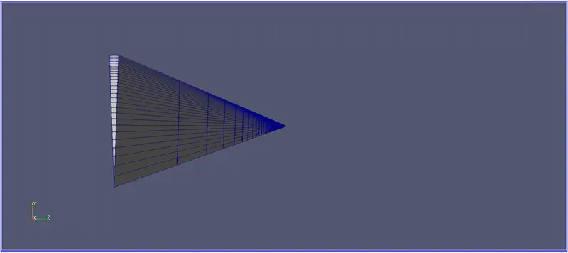
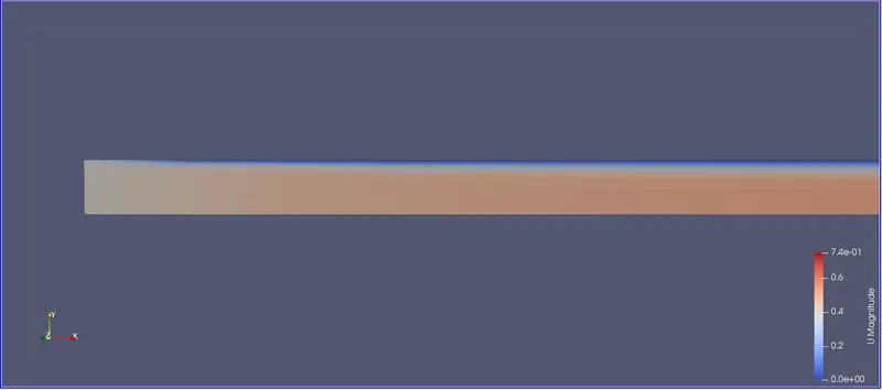
Inlet: We can see the developing flow at the inlet of the pipe.

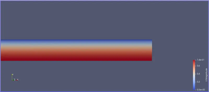
Outlet: We can see fully developed flow at the outlet of the pipe.

Output Graphs:

For angle `4^0`:

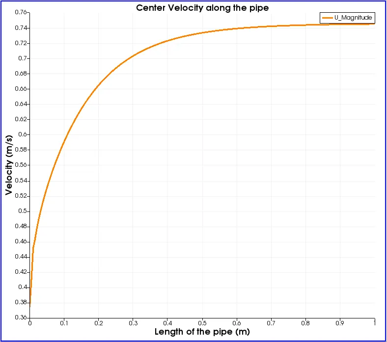
Velocity distribution along the pipe length:

Pressure drop along the length of the pipe:

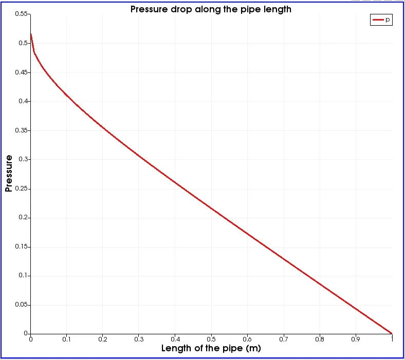
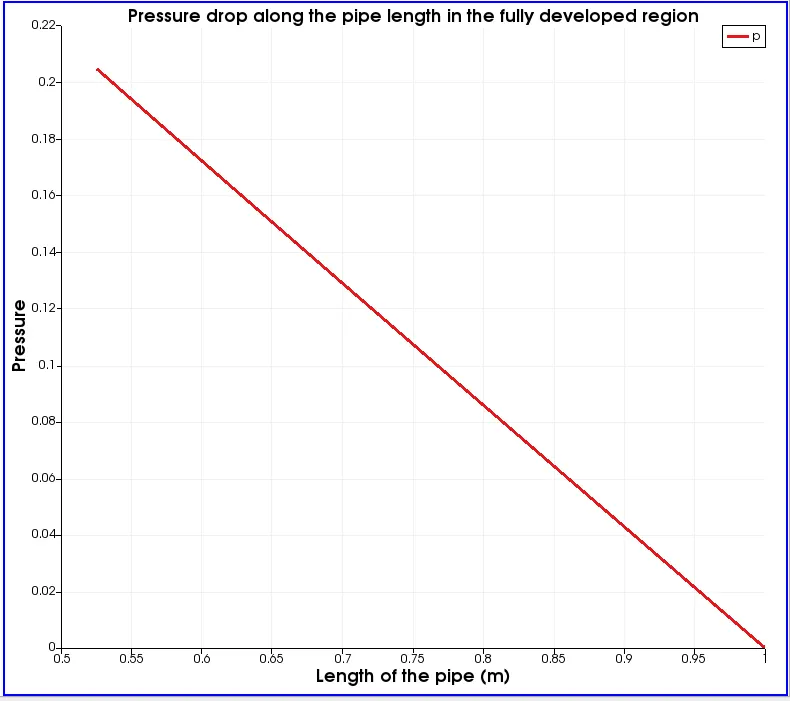
According to the Hagen-Poiseuile equation,

`Delta P = (32muLv)/(D^2)`

`DeltaP = (32*8.89*10^-4*1*0.374514)/(0.005^2) = 426.1669 (kg)/(m*s^2)`

Kinematic Pressure `P/rho`

KInematic pressure drop `(DeltaP)/rho = 426.1669/997 = 0.4274 m^2/s^2`

Velocity profiles at different lengths along the center of pipe from inlet:

For angle `4^0`:

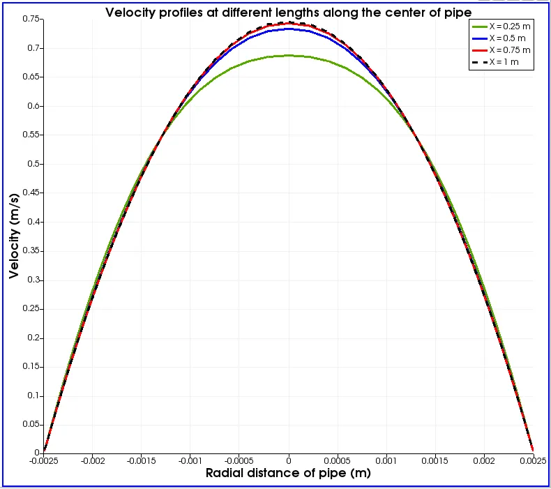
It is observed that the velocity profile gradually increased from the inlet to the outlet. we can see the maximum velocity at the outlet of the pipe.

This region is called a fully developed region. we can see velocity profile is completely developed at the outlet. The developing flow can be clearly seen from x = 0.25 to x = 0.5 m. and further along the length of the pipe.

The maximum velocity along the centerline for fully developed is, 2 times inlet velocity,

`U_(max) = 2*U = 2*0.374514 = 0.749028 m/s.`

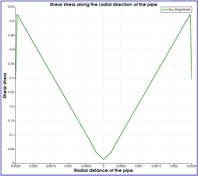
Shear stress variation from outer walls to the center of the pipe:

For angle `4^0`:

CASE 2: SYMMETRY BOUNDARY CONDITIONS

Octave Code:

clear all
close all
clc

% length of pipe
L = 1;

%wedge angle
theta = 45;

%Diameter of pipe
d = 0.005;
% Radius of pipe
r = d/2;

% reynolds number
Re = 2100;

% entrance length
Le = 0.05*Re*d;

% dynamic viscosity of water (NS/m^2)
mu = 8.89e-4;

%density (kg/m^3)
rho = 997;

% kinematic viscosity(m^2/s)
nu = mu/rho;

%average velocity(m/s)
V_avg = Re*nu/d;

% maximum velocity
V_max = 2*V_avg;

%Kinematic pressure drop (N/m^2)
delta_p = 32*nu*V_avg*L/d^2;

% radius
R = linspace(0,0.0025,30);

for i = 1:length(R)
  
  tau(i) = 16*mu*V_avg*R(i)/d^2;
  u(i) = 2*V_avg*(1-(R(i)^2/r^2));
end

figure (1)
plot (R,tau)
xlabel('Radius')
ylabel('wall shear stress')
legend('Analytical Wall shear stress profile')

figure (2)
plot (R,u)
xlabel('Radius')
ylabel('Velocity')
legend('Analytical Velocity profile')

nx = 200;
ny = 30;
nz = 7;


line1='/*---------------------------------*- C++ -*---------------------------------------*\';
line2='|  =========                 |                                                      |';
line3='|  \\      /  F ield         |  OpenFOAM: The Open Source CFD Toolbox               |';
line4='|   \\    /   O peration     |  Web:      https://openfoam.org                      |';            
line5='|    \\  /    A nd           |  Version:  8                                         |';        
line6='|     \\/     M anipulation  |                                                      |';              
line7='\*---------------------------------------------------------------------------------*/';

line8='//*********************************************************************************//';

f1 = fopen('blockMesh_symmetry.txt','w')
fprintf(f1,'%s\n',line1);
fprintf(f1,'%s\n',line2);
fprintf(f1,'%s\n',line3);
fprintf(f1,'%s\n',line4);
fprintf(f1,'%s\n',line5);
fprintf(f1,'%s\n',line6);
fprintf(f1,'%s\n',line7);


fprintf(f1,'FoamFile\n{\n');
fprintf(f1,'%12s \t 2.0;\n','version');
fprintf(f1,'%11s \t ascii;\n','format');
fprintf(f1,'%10s \t dictionary;\n','class');
fprintf(f1,'%11s \t blockMeshDict;\n','object');
fprintf(f1,'}\n');

fprintf(f1,'%s\n\n',line8);

fprintf(f1,'convertToMeters 1;\n\n');

fprintf(f1,'vertices\n');
fprintf(f1,'(\n');
fprintf(f1,'\t (%d %d %d)\n',0,0,0);                               % point 0
fprintf(f1,'\t (%d %d %d)\n',0,r*cosd(theta/2),r*sind(theta/2));   % point 1
fprintf(f1,'\t (%d %d %d)\n',0,r*cosd(theta/2),-r*sind(theta/2));  % point 2
fprintf(f1,'\t (%d %d %d)\n',L,0,0);                               % point 3
fprintf(f1,'\t (%d %d %d)\n',L,r*cosd(theta/2),r*sind(theta/2));   % point 4
fprintf(f1,'\t (%d %d %d)\n',L,r*cosd(theta/2),-r*sind(theta/2));  % point 5
fprintf(f1,');\n\n');

fprintf(f1,'blocks\n');
fprintf(f1,'(\n');
fprintf(f1,'\t hex (0 3 5 2 0 3 4 1) (%d %d %d)',nx,ny,nz);
fprintf(f1,' SimpleGrading (1 0.1 1)\n\n');
fprintf(f1,');\n\n');

fprintf(f1,'edges\n(\n\tarc %d %d (%d %d %d)\n',2,1,0,r,0);
fprintf(f1,'\tarc %d %d (%d %d %d)\n',5,4,L,r,0);
fprintf(f1,');\n\n');

fprintf(f1,'boundary\n(\n');
fprintf(f1,'\t inlet\n');
fprintf(f1,'\t{\n');
fprintf(f1,'\t\t type patch;\n');
fprintf(f1,'\t\t faces\n');
fprintf(f1,'\t\t (\n');
fprintf(f1,'\t\t\t (0 1 2 0)\n');
fprintf(f1,'\t\t );\n');
fprintf(f1,'\t}\n');

fprintf(f1,'\t outlet\n');
fprintf(f1,'\t{\n');
fprintf(f1,'\t\t type patch;\n');
fprintf(f1,'\t\t faces\n');
fprintf(f1,'\t\t (\n');
fprintf(f1,'\t\t\t (3 5 4 3)\n');
fprintf(f1,'\t\t );\n');
fprintf(f1,'\t}\n');

fprintf(f1,'\t top\n');
fprintf(f1,'\t{\n');
fprintf(f1,'\t\t type wall;\n');
fprintf(f1,'\t\t faces\n');
fprintf(f1,'\t\t (\n');
fprintf(f1,'\t\t\t (1 4 5 2)\n');
fprintf(f1,'\t\t );\n');
fprintf(f1,'\t}\n');

fprintf(f1,'\t back\n');
fprintf(f1,'\t{\n');
fprintf(f1,'\t\t type symmetry;\n');
fprintf(f1,'\t\t faces\n');
fprintf(f1,'\t\t (\n');
fprintf(f1,'\t\t\t (0 2 5 3)\n');
fprintf(f1,'\t\t );\n');
fprintf(f1,'\t}\n');

fprintf(f1,'\t front\n');
fprintf(f1,'\t{\n');
fprintf(f1,'\t\t type symmetry;\n');
fprintf(f1,'\t\t faces\n');
fprintf(f1,'\t\t (\n');
fprintf(f1,'\t\t\t (0 3 4 1)\n');
fprintf(f1,'\t\t );\n');
fprintf(f1,'\t}\n');

fprintf(f1,'\t axis\n');
fprintf(f1,'\t{\n');
fprintf(f1,'\t\t type empty;\n');
fprintf(f1,'\t\t faces\n');
fprintf(f1,'\t\t (\n');
fprintf(f1,'\t\t\t (0 3 3 0)\n');
fprintf(f1,'\t\t );\n');
fprintf(f1,'\t}\n');
fprintf(f1,');\n\n');

fprintf(f1,'mergePatchPairs\n(\n');
fprintf(f1,');\n');

fprintf(f1,'%s\n',line8);

fclose(f1)

blockMeshDict Files:

For wedge angle 10:

/*---------------------------------*- C++ -*---------------------------------------*\
|  =========                 |                                                      |
|  \\      /  F ield         |  OpenFOAM: The Open Source CFD Toolbox               |
|   \\    /   O peration     |  Web:      https://openfoam.org                      |
|    \\  /    A nd           |  Version:  8                                         |
|     \\/     M anipulation  |                                                      |
\*---------------------------------------------------------------------------------*/
FoamFile
{
     version 	 2.0;
     format 	 ascii;
     class 	 dictionary;
     object 	 blockMeshDict;
}
//*********************************************************************************//

convertToMeters 1;

vertices
(
	 (0 0 0)
	 (0 0.00249049 0.000217889)
	 (0 0.00249049 -0.000217889)
	 (1 0 0)
	 (1 0.00249049 0.000217889)
	 (1 0.00249049 -0.000217889)
);

blocks
(
	 hex (0 3 5 2 0 3 4 1) (200 30 3) SimpleGrading (1 0.1 1)

);

edges
(
	arc 2 1 (0 0.0025 0)
	arc 5 4 (1 0.0025 0)
);

boundary
(
	 inlet
	{
		 type patch;
		 faces
		 (
			 (0 1 2 0)
		 );
	}
	 outlet
	{
		 type patch;
		 faces
		 (
			 (3 5 4 3)
		 );
	}
	 top
	{
		 type wall;
		 faces
		 (
			 (1 4 5 2)
		 );
	}
	 back
	{
		 type symmetry;
		 faces
		 (
			 (0 2 5 3)
		 );
	}
	 front
	{
		 type symmetry;
		 faces
		 (
			 (0 3 4 1)
		 );
	}
	 axis
	{
		 type empty;
		 faces
		 (
			 (0 3 3 0)
		 );
	}
);

mergePatchPairs
(
);
//*********************************************************************************//

For wedge angle 25:

/*---------------------------------*- C++ -*---------------------------------------*\
|  =========                 |                                                      |
|  \\      /  F ield         |  OpenFOAM: The Open Source CFD Toolbox               |
|   \\    /   O peration     |  Web:      https://openfoam.org                      |
|    \\  /    A nd           |  Version:  8                                         |
|     \\/     M anipulation  |                                                      |
\*---------------------------------------------------------------------------------*/
FoamFile
{
     version 	 2.0;
     format 	 ascii;
     class 	 dictionary;
     object 	 blockMeshDict;
}
//*********************************************************************************//

convertToMeters 1;

vertices
(
	 (0 0 0)
	 (0 0.00244074 0.000541099)
	 (0 0.00244074 -0.000541099)
	 (1 0 0)
	 (1 0.00244074 0.000541099)
	 (1 0.00244074 -0.000541099)
);

blocks
(
	 hex (0 3 5 2 0 3 4 1) (200 30 5) SimpleGrading (1 0.1 1)

);

edges
(
	arc 2 1 (0 0.0025 0)
	arc 5 4 (1 0.0025 0)
);

boundary
(
	 inlet
	{
		 type patch;
		 faces
		 (
			 (0 1 2 0)
		 );
	}
	 outlet
	{
		 type patch;
		 faces
		 (
			 (3 5 4 3)
		 );
	}
	 top
	{
		 type wall;
		 faces
		 (
			 (1 4 5 2)
		 );
	}
	 back
	{
		 type symmetry;
		 faces
		 (
			 (0 2 5 3)
		 );
	}
	 front
	{
		 type symmetry;
		 faces
		 (
			 (0 3 4 1)
		 );
	}
	 axis
	{
		 type empty;
		 faces
		 (
			 (0 3 3 0)
		 );
	}
);

mergePatchPairs
(
);
//*********************************************************************************//

For wedge angle 45:

/*---------------------------------*- C++ -*---------------------------------------*\
|  =========                 |                                                      |
|  \\      /  F ield         |  OpenFOAM: The Open Source CFD Toolbox               |
|   \\    /   O peration     |  Web:      https://openfoam.org                      |
|    \\  /    A nd           |  Version:  8                                         |
|     \\/     M anipulation  |                                                      |
\*---------------------------------------------------------------------------------*/
FoamFile
{
     version 	 2.0;
     format 	 ascii;
     class 	 dictionary;
     object 	 blockMeshDict;
}
//*********************************************************************************//

convertToMeters 1;

vertices
(
	 (0 0 0)
	 (0 0.0023097 0.000956709)
	 (0 0.0023097 -0.000956709)
	 (1 0 0)
	 (1 0.0023097 0.000956709)
	 (1 0.0023097 -0.000956709)
);

blocks
(
	 hex (0 3 5 2 0 3 4 1) (200 30 7) SimpleGrading (1 0.1 1)

);

edges
(
	arc 2 1 (0 0.0025 0)
	arc 5 4 (1 0.0025 0)
);

boundary
(
	 inlet
	{
		 type patch;
		 faces
		 (
			 (0 1 2 0)
		 );
	}
	 outlet
	{
		 type patch;
		 faces
		 (
			 (3 5 4 3)
		 );
	}
	 top
	{
		 type wall;
		 faces
		 (
			 (1 4 5 2)
		 );
	}
	 back
	{
		 type symmetry;
		 faces
		 (
			 (0 2 5 3)
		 );
	}
	 front
	{
		 type symmetry;
		 faces
		 (
			 (0 3 4 1)
		 );
	}
	 axis
	{
		 type empty;
		 faces
		 (
			 (0 3 3 0)
		 );
	}
);

mergePatchPairs
(
);
//*********************************************************************************//

Results:

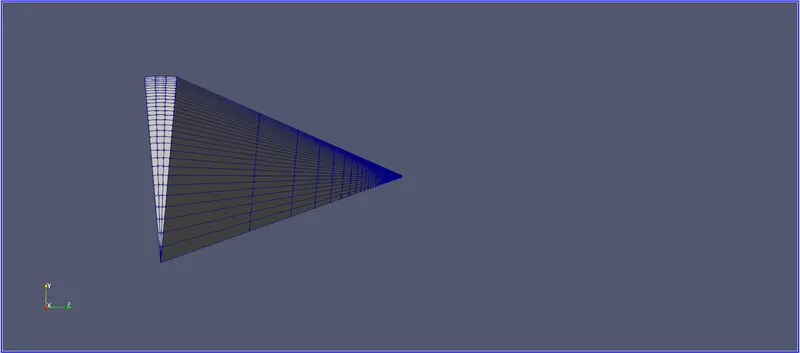
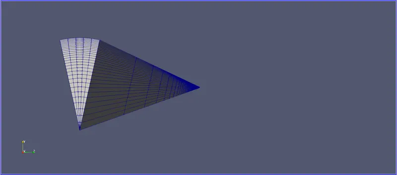
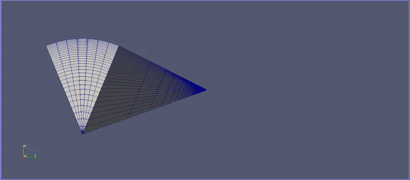
Mesh:

For `theta = 10`

For `theta = 25`

For `theta = 45`

Inlet: We can see the developing flow at the inlet of the pipe.

For angle `10^0`

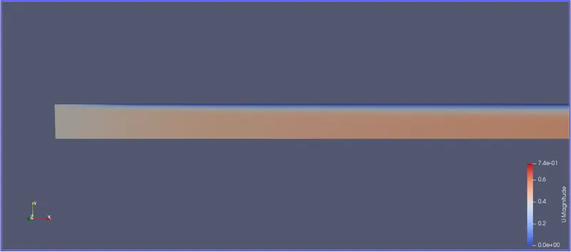
For angle `25^0`

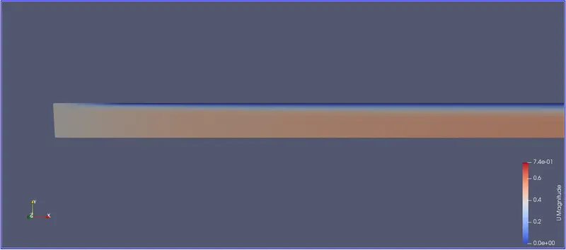
For angle `45^0`

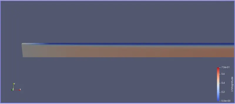
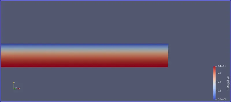
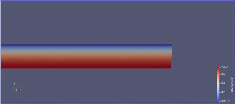
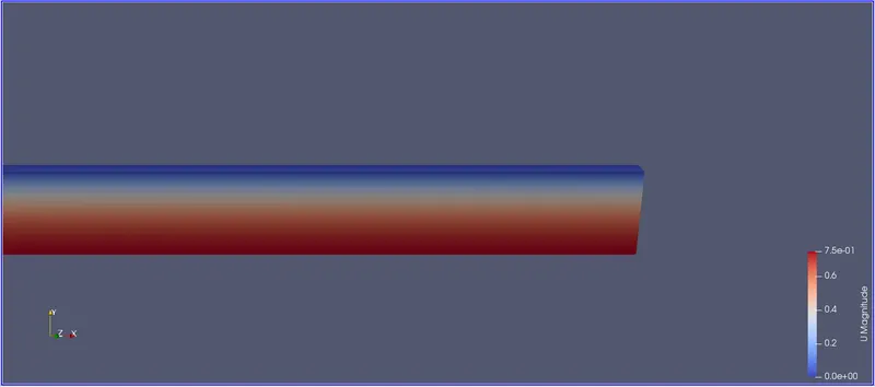
Outlet: We can see fully developed flow at the outlet of the pipe.

For angle `10^0`

For angle `25^0`

For angle `45^0`

Output Graphs:

For angle `10^0`

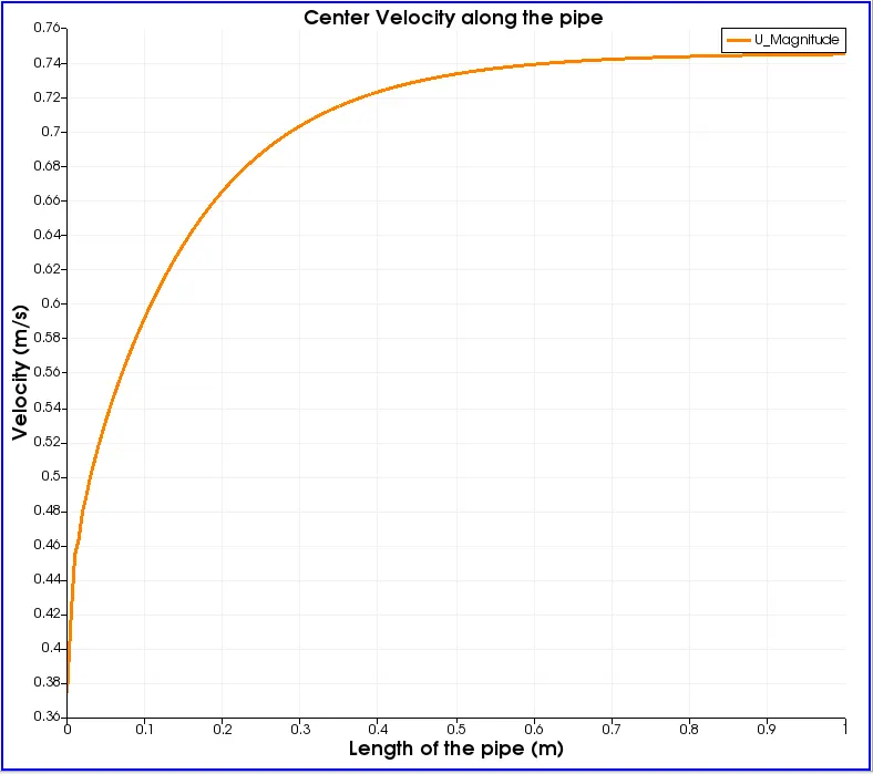
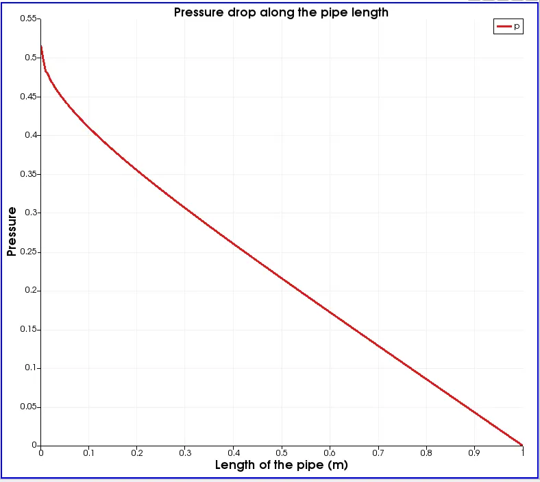
Velocity distribution along the pipe length:

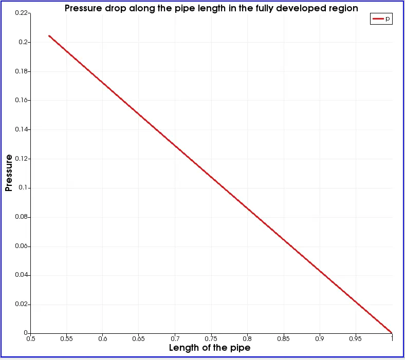
Pressure drop along the length of the pipe:

For angle `25^0`

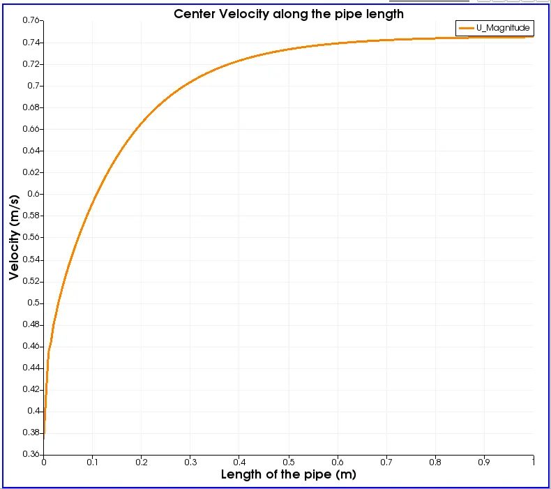
Velocity distribution along the pipe length:

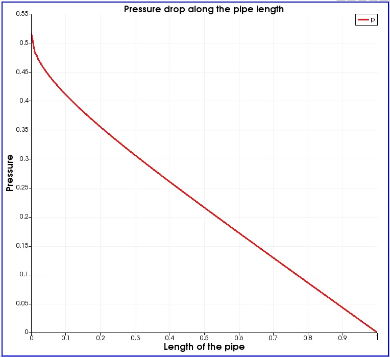
Pressure drop along the length of the pipe:

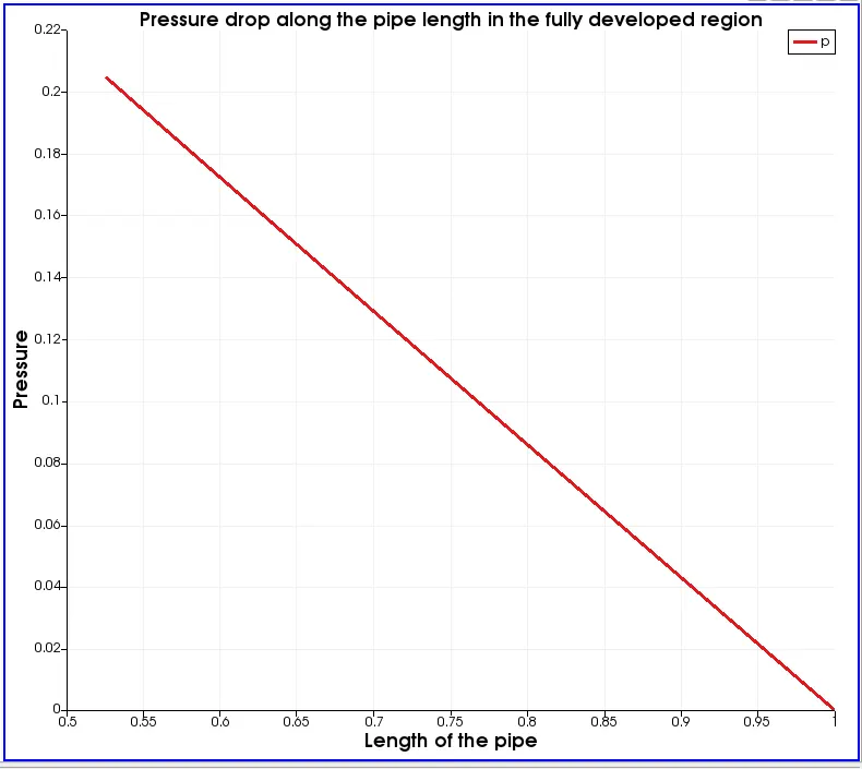
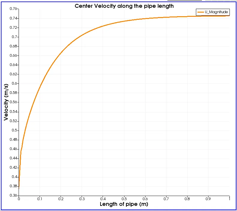
For angle `45^0`

Velocity distribution along the pipe length:

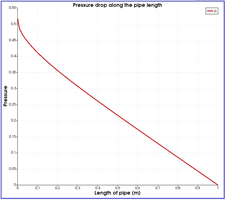
Pressure drop along the length of the pipe:

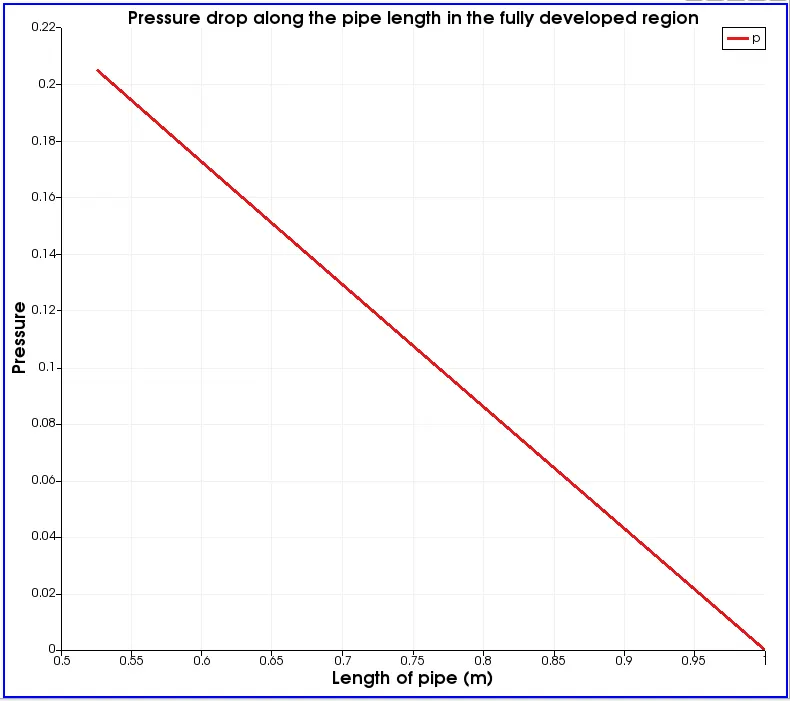
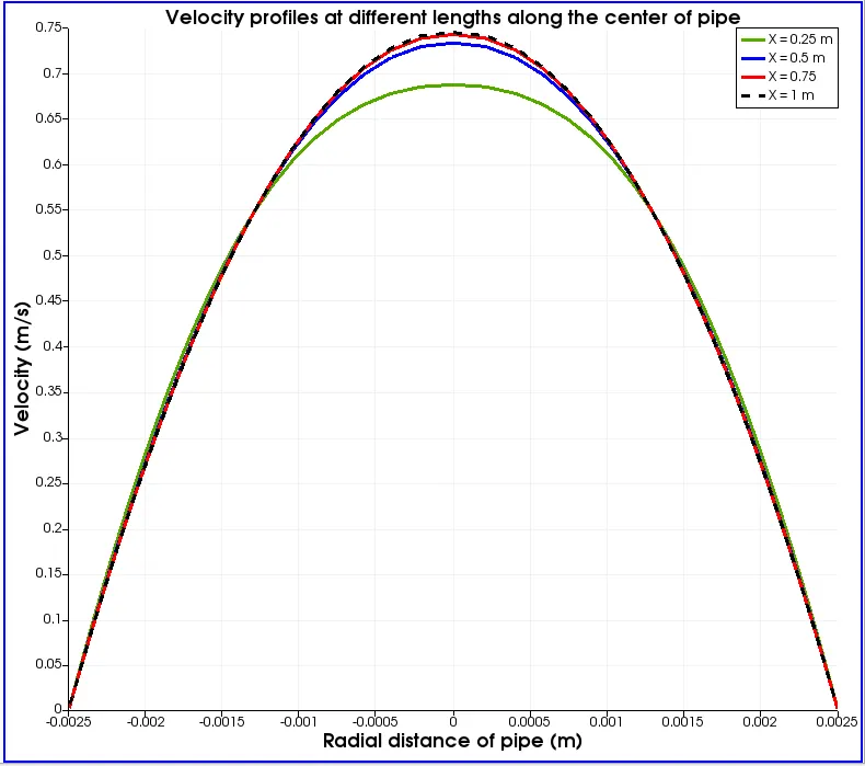
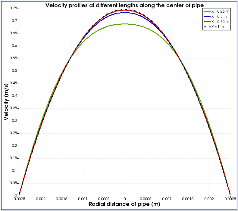
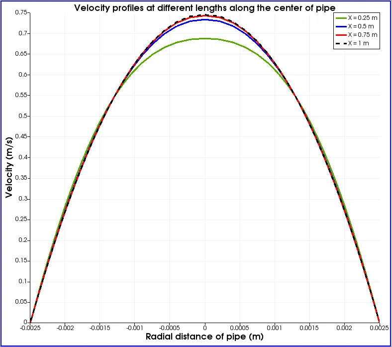
Velocity profiles at different lengths along the center of pipe from inlet:

For angle `10^0`:

For angle `25^0`:

For angle `45^0`:

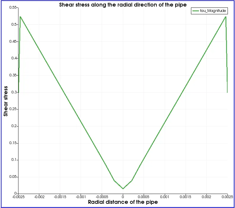
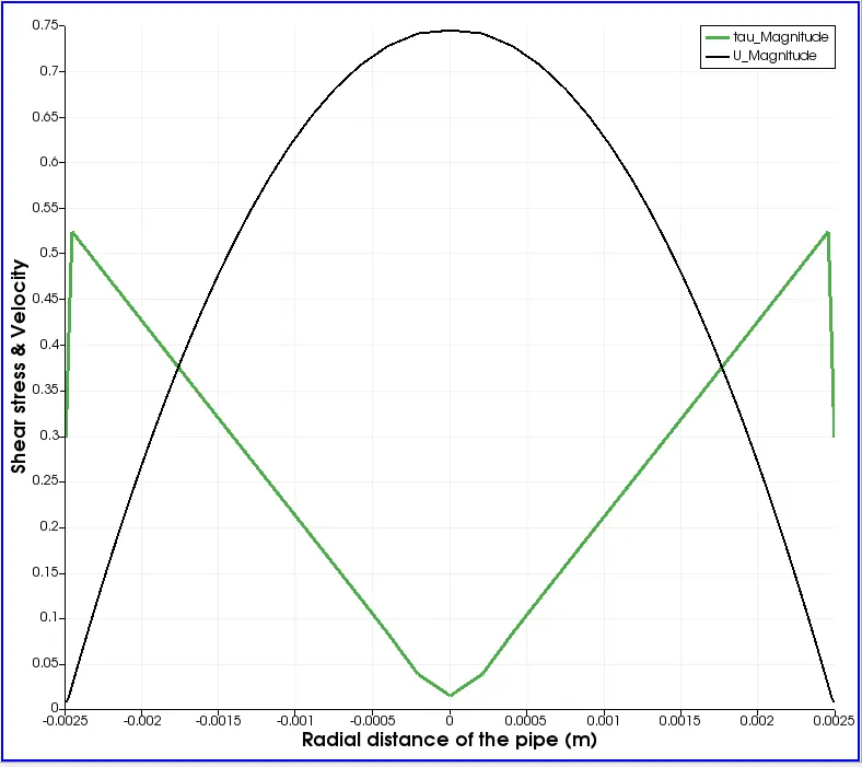
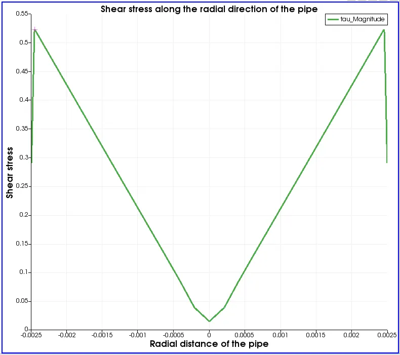
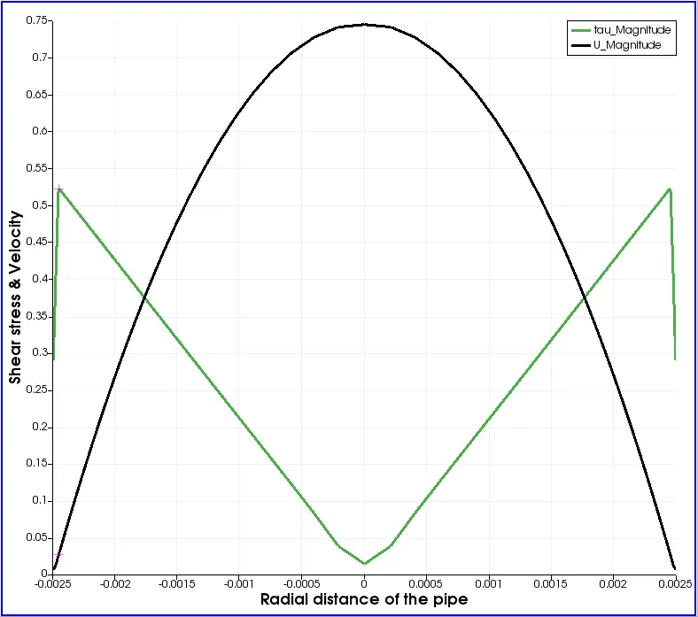
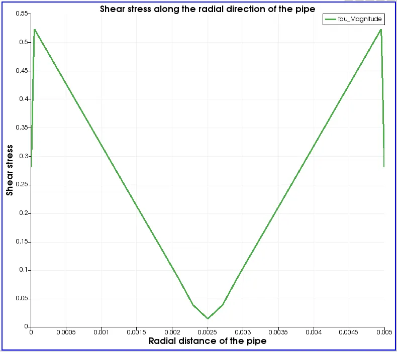
Shear stress variation from outer walls to the center of the pipe:

For angle `10^0`

For angle `25^0`:

For angle `45^0`:

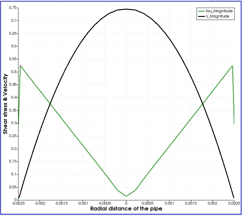
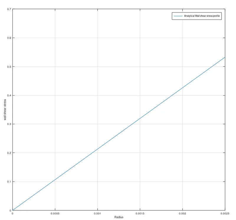
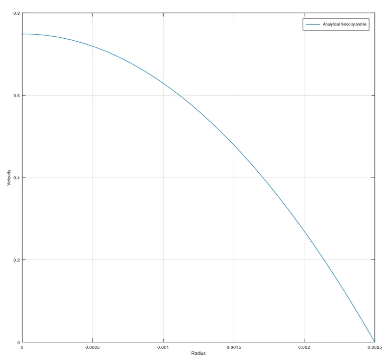
Analytically Calculated Shear Stress and Velocity Profiles:

Observations:

On Velocity Profiles:

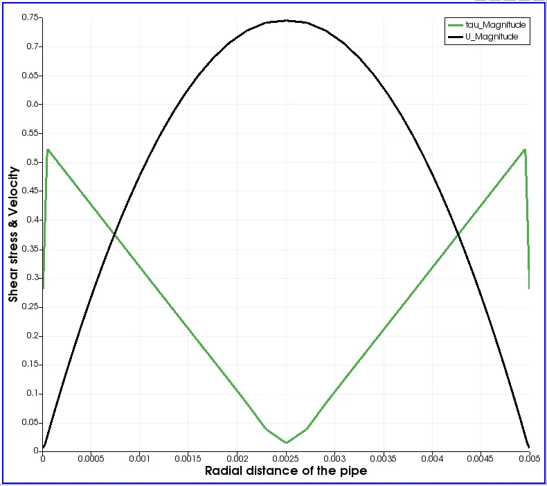
It is observed in the velocity profiles that the velocity profile gradually increased from the inlet to the outlet. We can see the maximum velocity at the outlet of the pipe.
The maximum velocity is at the center of the pipe and the minimum velocity at the surface.
we can see velocity profile is completely developed at the outlet. The developing flow can be seen from x=0.25 to x=0.5m.

On Shear Stress Profiles:

From the shear stress plots, we can infer that the shear stress is maximum at the walls due to the viscosity of the fluid and decreases along the radial direction of the pipe, and is zero at the center of the pipe.

On Pressure Profiles:

Pressure is maximum at the inlet and tends to zero at the outlet.

Comparison of the Results:

Results from Wedge Boundary Conditions:

Wedge Angle (Degree)	Maximum Velocity (Numerical Solution)	Maximum Velocity (Analytical Solution)	Maximum Shear Stress (Numerical Solution)	Maximum Shear Stress (Analytical Solution)	Execution Time (sec)	Courant Number (mean)	Courant Number (max)
4	0.744991	0.74903	0.5237	0.53269	198.07	0.0765122	0.302457

Results from Symmetry Boundary Conditions:

Wedge Angle (Degree)	Maximum Velocity (Numerical Solution)	Maximum Velocity (Analytical Solution)	Maximum Shear Stress (Numerical Solution)	Maximum Shear Stress (Analytical Solution)	Execution Time (sec)	Courant Number (mean)	Courant Number (max)
10	0.744993	0.74903	0.524117	0.53269	2774.91	0.0765126	0.30213
25	0.744996	0.74903	0.523078	0.53269	3199.08	0.0765126	0.302036
45	0.745	0.74903	0.523089	0.53269	4635.44	0.0765124	0.302109

Conclusion:

Here we can see that as the wedge angle increases the velocity becomes more accurate to the analytical value.
We observe that the symmetry boundary condition is more accurate in terms of velocity where it is very close to the true value.
We can say symmetry boundary conditions give more accurate results than wedge boundary conditions.
Symmetry boundary conditions take more execution time than wedge boundary conditions. As in the case of symmetry boundary condition, the calculation across the arc of the wedge is done hence the simulation time is higher in that case.
As the wedge angle increases the courant number increase because it increases the element size of the mesh. As the Courant number is directly proportional to the element size.
In conclusion, we can say that the wedge boundary condition is applicable only for wedge shape geometry but the symmetry boundary condition can be used for any geometry as there are no wedge angle restrictions.

Week 12 - Validation studies of Symmetry BC vs Wedge BC in OpenFOAM vs Analytical H.P equation

Ship work like this
in your own course.

Talk to a career counsellor

Ship work like thisin your own course.

Talk to a career counsellor

Ship work like this
in your own course.