Week 6 Challenge-FVM Fundamentals 101

1.  Derive the expression for the ∂f/∂x for a forward difference of second order.

To derive the expression for a forward difference of second order of ∂f/∂x by using Taylor's series expansion. We know that the Taylor's series expansion for a function f(x) about a point x is 

`f(x+h) = f(x) + h * (∂f) / (∂x) + (h^2/(2!)) * (∂^2f)/(∂x^2) + (h^3/(3!)) * (∂^3f)/(∂x^3) + ...`

Here, the h is a small step size in the x-direction.

Now, let's consider the forward difference at the first order:

`(∂f)/(∂x) = [f(x+h)-f(x)]/h`

To get the forward difference of the second order, we can approximate the second-order derivative term in the Taylor series expansion.

The term `(h^2/(2!)) * (∂^2f)/(∂x^2)` can be approximated as follows:

`(h^2/(2!)) * (∂^2f)/(∂x^2) = (f(x + 2h) - 2f(x + h) + f(x)) / h^2`

Now, we can subtract this second-order approximation from the first-order forward difference to obtain the forward difference of the second order:

Forward Difference (2nd order) = `[f(x + h) - 2f(x) + f(x - h)] / h^2`

So, the expression for the forward difference of the second order (∂f/∂x) is:

`(∂f)/(∂x) = [f(x + h) - 2f(x) + f(x - h)] / h^2`

This expression is an approximation of the second derivative of the function f(x) using the forward difference method with a step size of h.

    2. Apply Finite Volume Formulation to the equation`(∂ ρ ϕ)/( ∂ t) + ∇ . ( ρ u ϕ ) = 0`

The given Differential Equation is  `(∂ ρ ϕ)/( ∂ t) + ∇ . ( ρ u ϕ ) = 0` --------> eq(1)

By, using Gauss Divergence Theorem we can formulate the volume integral apppering in the governing equation into surface intergral. This theorem simply states that the outward flux of a vector field through a closed surface is equals to the volume integral of the divergence over the region inside the surface.

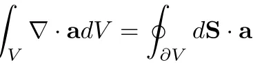
where, ∂V_p is a closed surface bounding the control volume V_p and dS represents an infinitesimal surface elements with associated normal n pointing outwards of the surface ∂V_p and ndS = dS

Applying this theorem to eq1 we get,

`∫(∂ ρ ϕ)/( ∂ t) + ∫∇ . ( ρ u ϕ ) = 0`

Multiply dv on both sides, we get

`∫((∂ ρ ϕ)/( ∂ t)) dv+ ∫∇ . ( ρ u ϕ ) dv= 0` 

Again by appling gauss divergence

`(∂ /( ∂ t)) ∫<sub>v</sub>ρ ϕdV + ∫ ρ ϕU.dS = 0`

i.e.., `∫<sub>s</sub> ρ ϕU.dS = ∑<sub>f</sub> S<sub>f</sub> (ρ ϕU)<sub>f</sub> `

this also written as  

`∂ /( ∂ t) ∫_vρ ϕdV = ∑_f S_f (ρ ϕU)_f  

the left hand side term is the convection term and the right hand side terms is, where we have approximated the integrant by means of the mid point rule, which is second order accurate.

     3. Note on the van Leer TVD scheme 

The Van Leer Total Variation Diminishing (TVD) scheme is a numerical method used for solving hyperbolic partial differential equations (PDEs), particularly in the context of computational fluid dynamics (CFD). The TVD scheme was developed to maintain the Total Variation of a solution, which is a measure of the smoothness of the solution, and to prevent unphysical oscillations in the presence of discontinuities.

The scheme is named after the Dutch mathematician Bram Van Leer. To understand the Van Leer TVD scheme, it's helpful to use the Sweby Diagram, which provides insights into the scheme's behavior in terms of stability and TVD property. The Sweby Diagram is a graphical tool that helps determine the allowable Courant-Friedrichs-Lewy (CFL) number for a given TVD scheme to ensure it remains TVD.

TVD Property:

• TVD schemes are designed to preserve the total variation of a solution, meaning they minimize spurious oscillations while maintaining sharp discontinuities.
• The desirable property for a stable, non-oscillatory, higher order scheme is monotonicity preserving.
• In simple terms, monotonicity-preserving schemes do not create new undershoots and overshoots in the solution or accentuate existing extremes.
• Monotonicity-preserving schemes have implications for the so-called total variation of discretised solutions.Monotonicity-preserving schemes have implications for the so-called total variation of discretised solutions. 
• For monotonicity to be satisfied, TV must not increase. 

The Sweby Diagram:

• The Sweby Diagram is a plot of the maximum amplification factor (y-axis) against the Courant-Friedrichs-Lewy (CFL) number (x-axis).
• The Sweby Diagram shows the region in which the TVD scheme remains TVD (total variation diminishing) for different slope limiters.

Limited linear schemes

The limited linear scheme — as the name suggests — maintains the linear scheme as much as possible to be TVD, before limiting to upwind to improve boundedness. Limited linear is a robust scheme that exhibits low diffusion, but has a disadvantage that it is not symmetric.