Calculate the Stretch Ratio by comparing the ELFORM (-2, -1, 1, 2) with Ogden_Material Model.
INTRODUCTION
Two terms are frequently used when the properties of the material are discussed. One is the Poisson’s ratio, which defines the limit of stretching or deforming a material before failure, and the strain, which defines that how much the material has already been deformed due to applied load. But, in the case of elastomers or the material which can be highly stretched, there is one more term of dramatic importance, and i.e., a stretch ratio. The stretch ratio is the measure of the extension of the material. It is the ratio of the final length and the initial length of the material. In this work, an Ogden material model was applied to a cubical box, under uniaxial tension, to see the difference that results when the element formulation is changed. Four different element formulations were used i.e., -2, -1, 1, and 2, and thus four cases were studied.
OBJECTIVE
- To apply appropriate boundary conditions, to the cubical box, to which an Ogden material is defined, for the uniaxial tension.
- To use implicit solver for solving the problem.
- To evaluate the stretch ratio for the four cases, and compare the difference.
PROCEDURE
Pre-processing
In this work, a block had to undergo a tensile loading. To impose that boundary condition, initially, a block of 10 mm x 10 mm x 10 mm dimension, with 10 elements for each direction, was created, as can be seen in the figure below.
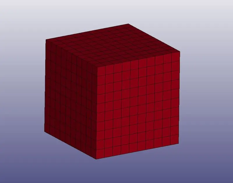
Figure 1: 10 mm x 10 mm x 10 mm block with 10 elements in each direction.
Secondly, this block has to be assigned with the material. The material that had to use in this work was hyperelastic material. Therefore, using the Keyword Manager → All → MAT → 077_O-OGDEN_RUBBER, a hyperelastic material card was created. The data to feed in that card was already available and thus was feed accordingly, as can be seen in fig. 2 below. This material card had MID or material ID, which was given to the available part. Thus, the material was assigned to the cubical block part.
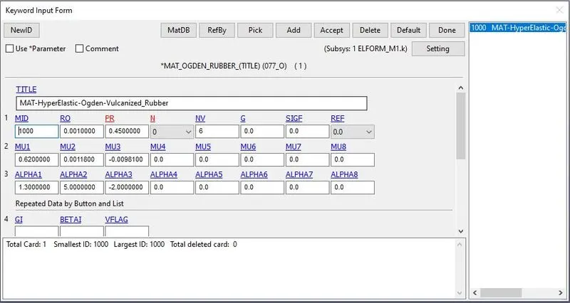
Figure 2: Material card for assigning a hyperelastic material.
After material, the section card had to define. Using section cards, the element formulation can be selected. In this work, four cases were divided based on the four different element formulations. Now, considering the first case i.e., element formulation or ELFORM = -2, the section card for the first case was created. This ELFORM ensures fully integrated S/R (selective reduced) solid intended for elements with poor aspect ratio, accurate formulation.
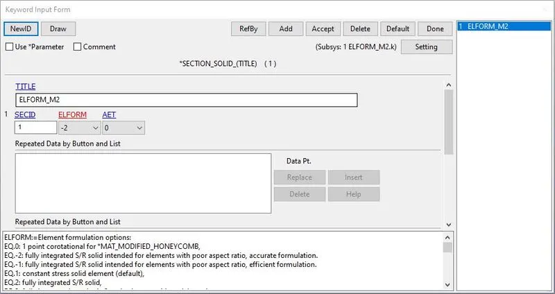
Figure 3: Section card to define the element formulation.
For, uniaxial loading, one face of the block had to fix in all directions, except its transverse direction, so the model would have 2 dof. It is required, to let the block model compress when it is stretched. Using Model and Part → Create Entity → Boundary → Spc, nodes of one face of the block were constrained in 4 dof.
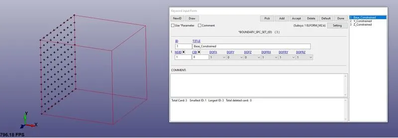
Figure 4: Nodes of one face of the block constrained to 4 of (movable in Y & Z directions).
Next, the model, should not move in the global Y and Z direction. Therefore, a node-set is constrained in Y- and Z-coordinate, as shown in the figure below.
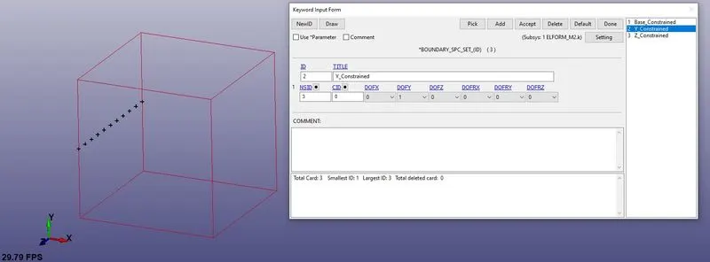
Figure 5(a): Nodes constrained in Y-direction of global coordinate.
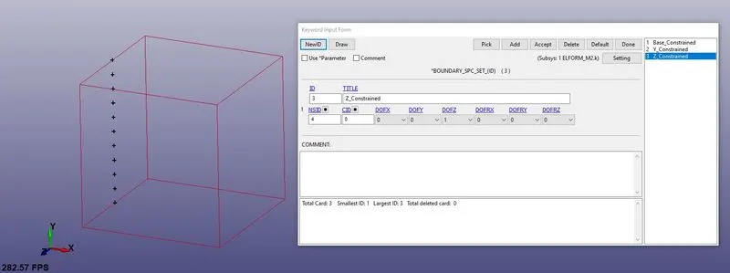
Figure 5(b): Nodes constrained in Z-direction of global coordinate.
And to the opposite face, a displacement had to impose. In this work, tensile loading had to apply on the hyperelastic block to a stretch ratio of 5.
Now,
Stretch Ratio = (final length / initial length) = (1 + engineering strain).
`⇒Stretch Ratio=1+(δL)/L`
`Stretch Ratio=5,`
`L=10`
`⇒Stretch Ratio=5=1+δL/10`
`⇒δL=40`
Thus, to get the stretch ratio of 5, 40 mm of displacement had to impose. To impose the displacement, firstly, a curve has to be defined. So, using Model and Part → Keyword Manager → All → DEFINE → CURVE, a displacement curve was created.
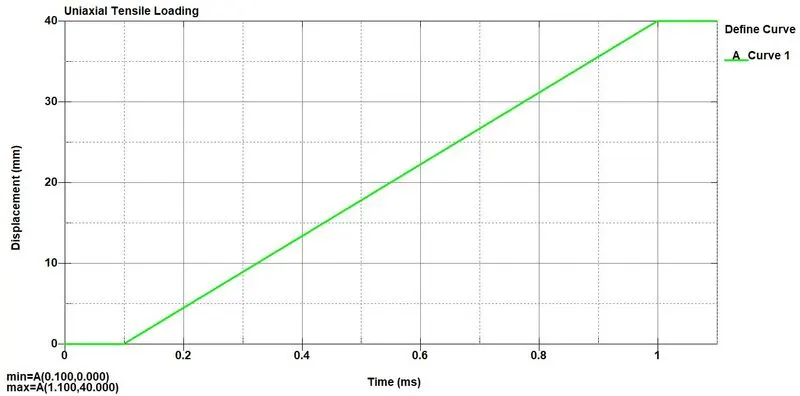
Figure 6: Displacement vs. Time curve.
For imposing the displacement, Model and Part → Create Entity → Boundary → Prescribed Motion was selected. In that, VAD was selected as 2, which ensures imposition of displacement, and to the LCID, the ID of the curve was provided that was created just before.
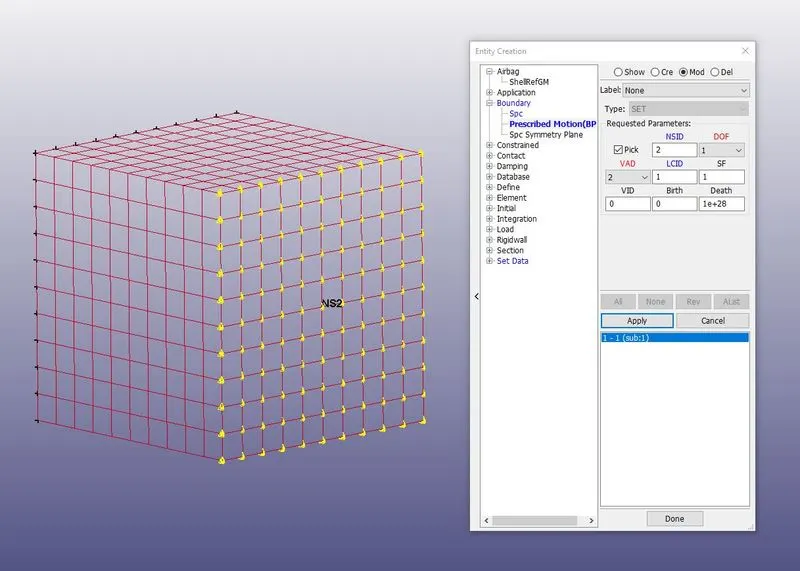
Figure 6: Displacement is given to the face, opposite to the fixed face, of the block.
This is how, the model was defined with the material, element formulation, and boundary condition. Now, the analysis had to run with an implicit solver. So, to activate the implicit solver, the CONTROL_IMPLICIT_GENERAL card was created, wherein IMFLAG was kept equal to 1, which activated the implicit mode of analysis. CONTROL_IMPLICIT_GENERAL card ensures that the analysis would run implicitly because the default mode of solving the analysis for LS-DYNA is explicit.
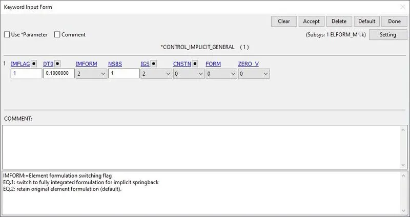
Figure 7: CONTROL_IMPLICIT_GENERAL card for activating implicit analysis.
After IMPLICT_GENERAL, the IMPLICIT_AUTO card was created. It is not a mandatory card to include, however, for learning it was included. It is used to control the time-step. In fig. 8, it can be observed that IAUTO was kept equal to 1. It ensures automatic control of time step size.
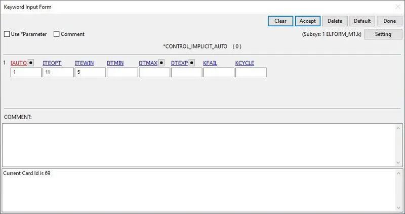
Figure 8: CONTROL_IMPLICIT_AUTO card to control time step.
A control card was required to control the simulation process. In this, the only essential card that was required was the termination card. It is used to define the termination time of the simulation. The termination time was set at 10.0 ms. It was defined using the Keyword Manager, picking the ‘All’ and selecting CONTROL → TERMINATION. In that card, the ENDTIM or the end time was given as 10.0.
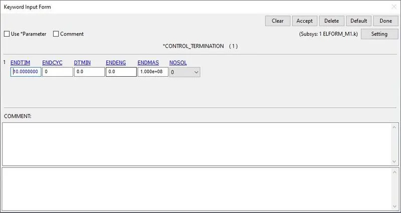
Figure 9: Termination card to define the total simulation time.
Database cards are required to command the software that what files are required as output. In this simulation, binary_d3plot was required to generate. So using Keyword Manager, and selecting the ‘All’, in the DATABASE, BINARY_D3PLOT was selected. In that card, DT was given as 0.01, which plots the results at every 0.01 milliseconds.
In the results, since the stretch ratio is the part of the concern, the DATABASE_HISTORY_NODE card was created, to check the deformation of the node. But it activates and provides the results only when the ASCII file is requested. Therefore, DATABASE_ASCII_option, NODOUT was activated, which provides the nodal information, in the results.
Once done with defining the keywords, the next essential thing is to check that if any errors are present in it. Therefore, using the Model Checking, the keywords were checked for errors and warnings. When no errors were found, the simulation was run.
After completing defining all the keywords, the model was saved in .k format.
In other cases, each step remained the same. The only thing that required change was the change of ELFORM, in the section card.
Post-processing
In post-processing, the result that was required was the stress vs. stretch ratio plot. It is because the only change that happened in every four cases was the change in ELFORM (element formulation. The change in element formulation in LS-DYNA, for incompressible material with solid 8-node element, leads to a change in behavior of calculating the stiffness of each element of the block.
The bulk modulus of the material is the resistance to compress when uniform pressure is applied in all directions. Analogous to Young’s modulus, it is the ratio of change in pressure to the change in volume. Bulk modulus, K, can also be written in form of Young’s modulus, E as:
`E=3K*(1-2μ)`
`⇒K=E/(3*(1-2μ))`
Where µ is the Poisson’s ratio.
Now, in the above equation, if the Poisson’s ratio is equal to 0.5, the value of K i.e., the bulk modulus becomes zero, which indicates a highly stiff property. Thus, anything with Poisson’s ratio tending to 0.5, leads to high stiffness. This is called the volumetric locking of the material, which can be found in incompressible material like rubber, with Poisson’s ratio close to 0.5. ( In this work, it is equal to 0.45). Volumetric locking can be imagined as rubber with stress but no strain.
When reduced integration elements are used it causes a hourglassing effect (non-physical, zero-mode of deformation). So, using fully integrated elements is a solution for this problem. However, they have disadvantages too. It is costlier than single-point integration, and they tend to shear lock.
In case 1, ELFORM -2 was chosen. It uses fully integrated S/R solid intended elements with poor aspect ratio, accurate formulation. The term S/R means Selective Reduced Integration. Thus, in stiffness calculation, the shear and volumetric integration are accomplished separately. Shear contributes to the change in shape with full integration, and the volume contributed to the change in volume with reduced integration. Due to the shear locking tendency of the fully integrated elements, it causes a poor aspect ratio. However, it is more efficient to use, considering the accuracy because of modified Jacobian, compared to ELFORM 2.
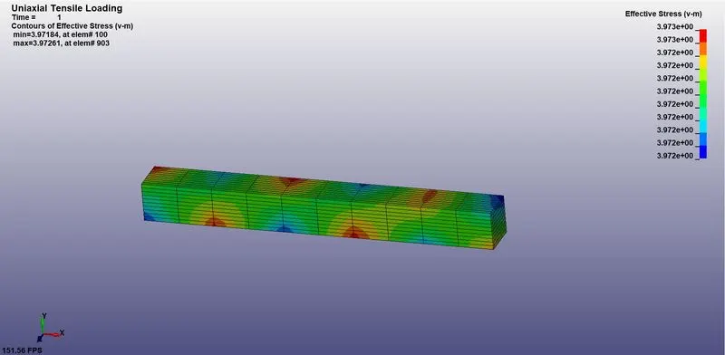
Figure 10: Von Mises Stress contour with a maximum stress of 3.97 MPa.
LS-Dyna calculates the stress and strain values, in terms of true stress and true strain. In this work, the objective was to plot engineering stress vs. stretch ratio plots. To plot this stress vs. stretch ratio plot, a series of data was required which were the true stress data, the true strain data, for any particular element. From these data, the engineering stress and engineering strain data can be evaluated as shown below.
True Stress = Engineering Stress*(1+Engineering Strain)
True Strain = ln(1+Engineering Strain)
Stretch Ratio = (Final Length)/(Original Length) = (1+Engineering Strain)
Now, taking the true stress and true strain data from the simulation, and using the formula above, the engineering stress and stretch ratio data were evaluated as shown below.
Table 1: Stress and Strain data for ELFORM = -1.
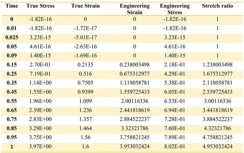
The plot of engineering stress vs. stretch ratio can be seen below, which was plot using the data shown above.
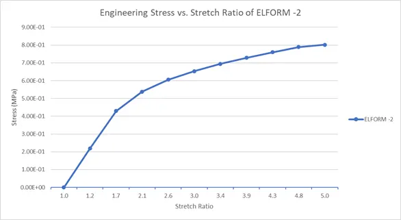
Figure 11: Stress vs. Stretch ratio plot for ELFORM = -2.
Similar to case I, the other cases were analyzed by changing the type of element formulation. Their Von Mises contours and the results of the stress vs. stretch ratio plot are shown below.
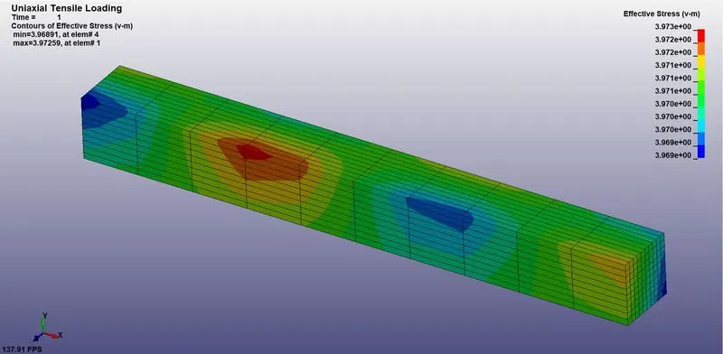
Figure 12: Von Mises contour with a maximum stress of 3.97 MPa.
Table 2: Stress and Strain data for ELFORM = -1.
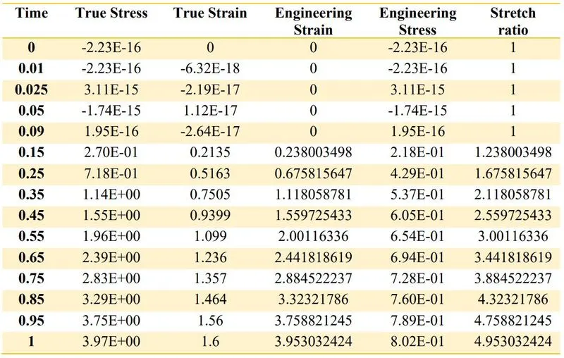
The plot of engineering stress vs. stretch ratio can be seen below, which was plot using the data shown above.
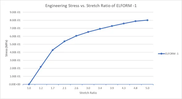
Figure 13: Stress vs. Stretch ratio plot for ELFORM = -1.
Case III
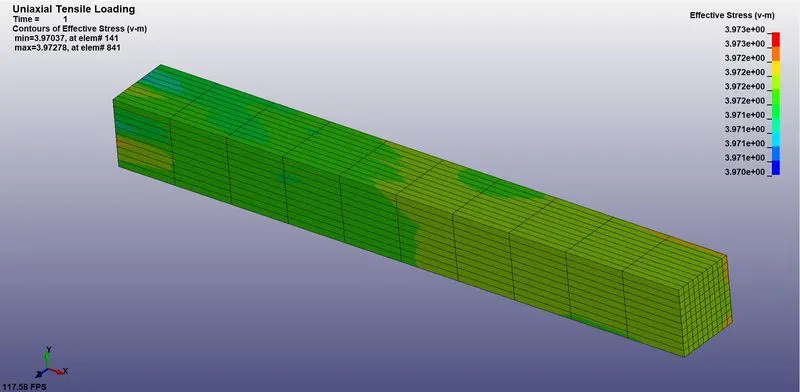
Figure 14: Von Mises contour for ELFORM = 1, with maximum stress of 3.97 MPa.
Table 3: Stress and Strain data for ELFORM = 1.
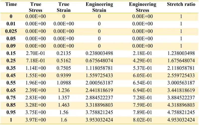
The plot of engineering stress vs. stretch ratio can be seen below, which was plot using the data shown above.
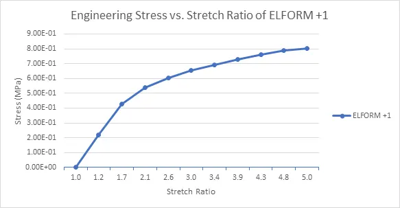
Figure 15: Stress vs. Stretch ratio plot for ELFORM = 1.
Case IV
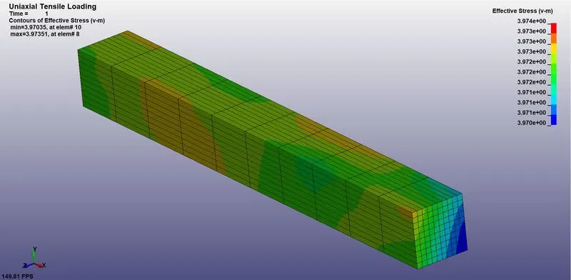
Figure 16: Von Mises contour for ELFORM = 2, with maximum stress of 3.97 MPa.
Table 4: Stress and Strain data for ELFORM = 2.
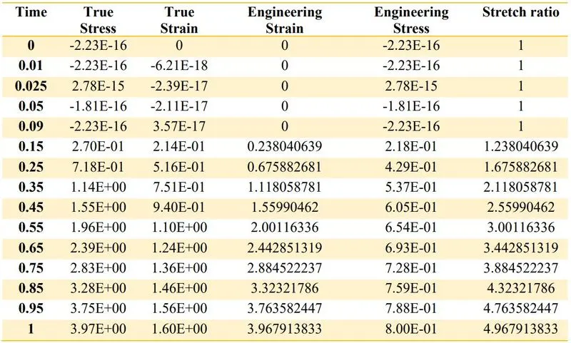
The plot of engineering stress vs. stretch ratio can be seen below, which was plot using the data shown above.
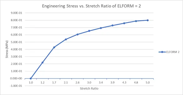
Figure 17: Stress vs. Stretch ratio plot for ELFORM = 2.
After observing the results of the four cases, it was difficult to identify the change in the result. It can be because of the simple uniaxial test of the material. ELFORM 1 defines the element with constant stress solid element. Due to this hourglass can induce in the element, and therefore, ELFORM 2, -2, or 1 are preferred. The ELFORM 2 defines the elements with fully integrated S/R solid elements. Now, due to full integration, an element can suffer shear locking, due to which its aspect ratio disturbs, and thus disturbs the formulation. To not let the formulation disturb, modified Jacobian is used in ELFORM -2, which gives accurate formulation, and ELFORM -1, which gives efficient formulation.
The above results were also tried to observe for the difference with one another, by merging them in a single plot. But as can be seen in fig. 18 below, no significant difference can be seen with the naked eye. The only difference that was observed from the tables is that ELFORM 2 is deviated from ELFORM 1 by 0.2% at the end of the simulation.
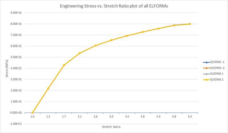
Figure 18: Stress vs. stretch ratio plot of all ELFORMs.
CONCLUSION
In this work, a hyperelastic block was subjected to a uniaxial tensile load with 4 different element formulations. Engineering stress vs. stretch ratio plot was drawn for all four cases, in which no significant difference was found, as expected. It might be because of the simple uniaxial tension, wherein no distortion has occurred in any element. But, the change in the formulation of constant stress to fully integrated S/R, has shown a change in the Von Mises contour, which can be observed in fig. 14, and fig. 16. The difference can also be observed between accurate formulation and efficient formulation, in fig. 10, and fig. 12, respectively. This shows that although the stress developed w.r.t. stretch ratio is the same, the stress distribution is not.