Week-6 Calculate the Stretch Ratio by comparing the ELFORM (-2,-1,1,2) with Ogden_Material Model.

INDEX

1. OBJECTIVE

• Deliverables

2. THEORY

• Engineering and True stress/ strain relations before the necking process.
• Stretch ratio (`λ`)
• Element formulation

3. DESIGN OF EXPERIMENT

• Type of loading
• Type of analysis
• Analysis solution design

4. CREATION OF SOLID CUBE ELEMENTS.

5. KEYWORDS

• *Material
• *Boundary
• *Control
• *Section
• *Part
• *Set
• *Database
• *Define

6. POST-PROCESSING

• CASE1: ELFORM = 1
• CASE2: ELFORM = -1
• CASE3: ELFORM = 2
• CASE4: ELFORM =-2

7. CONCLUSION

8. ATTACHMENTS

LIST OF TABLES

• Table 1.0: Displacement dependent loading with time
• Table 1.1: Data for Stresses/ Strain - Stretch ratio become > 5 at load step 3.5
• Table 1.2: Data for Stresses/ Strain - Stretch ratio become > 5 at load step 3.5
• Table 1.3: Data for Stresses/ Strain - Stretch ratio become > 5 at load step 3.5
• Table 1.4: Data for Stresses/ Strain - Stretch ratio become > 5 at load step 3.5

LIST OF FIGURES

• Figure 1.0: 10 x 10 x 10 mm3 comprising of 10 elements in x,y and z respectively.
• Figure 1.1: Front view for constraints.
• Figure 1.2: Vonimisses stress for Element formulation 1 (At final load step)
• Figure 1.3: Vonimisses stress for Element formulation -1 (At final load step)
• Figure 1.4: Vonimisses stress for Element formulation 2 (At final load step)
• Figure 1.5: Vonimisses stress for Element formulation -2 (At final load step)

LIST OF PLOTS

• Plot 1.0: Load curve data is loaded from XYdata option imported from XYDATA.csv file.
• Plot 1.1: Stress induced in z direction for element #661 Vs time.
• Plot 1.2: Strain induced in z direction for element #661 Vs time
• Plot 1.3: Engg stress and True stress Vs Stretch ratio for element formulation 1.
• Plot 1.4: Engg strain and True strain Vs Stretch ratio for element formulation 1.
• Plot 1.5: Stress induced in z direction for element #661 Vs time.
• Plot 1.6: Strain induced in z direction for element #661 Vs time.
• Plot 1.7: Engg stress and True stress Vs Stretch ratio for element formulation -1.
• Plot 1.8: Engg strain and True strain Vs Stretch ratio for element formulation -1.
• Plot 1.9: Stress induced in z direction for element #661 Vs time.
• Plot 1.10: Strain induced in z direction for element #661 Vs time.
• Plot 1.11: Engg stress and True stress Vs Stretch ratio for element formulation 2.
• Plot 1.12: Engg strain and True strain Vs Stretch ratio for element formulation 2.
• Plot 1.13: Stress induced in z direction for element #661 Vs time.
• Plot 1.14: Stress induced in z direction for element #661 Vs time.
• Plot 1.15: Engg stress and True stress Vs Stretch ratio for element formulation -2.
• Plot 1.16: Engg strain and True strain Vs Stretch ratio for element formulation -2.

_________________________________________________________________________________________

OBJECTIVE:

To create a 10 x 10 x 10 mm3 cube with 10 elements in each direction with Ogden_Material (MAT 77).

Solid elements need to be formulated as per following formulation:

1. ELFORM 1
2. ELFORM -1
3. ELFORM 2
4. ELFORM -2

Uniaxial tensile behaviour is to be studied till stretch ratio reaches 5.

Deliverables: (For each element formulation)

1. An excel sheet with proper conversion and calculation of Stress/Strain and the Stretch Ratio for all the ELFORM.
2. A proper image of the plot comparison of various ELFORMS against the Uniaxial Plot given in the challenge.

THEORY:

Engineering and True stress/ strain relations before the necking process.

`λ` : Stretch ratio

`ε`: Engineering strain

`ε`*: True strain

`sigma`: Engineering stress

`sigma`*: True stress

Relation between True stress and Engineering stress (Before necking in tensile loading)

`sigma`* = `sigma`(1 + `ε`)

so, `sigma` = `sigma`* / (1 + `ε`)

Relation between True strain and Engineering strain (Before necking in tensile loading)

`ε`* = ln (1 + `ε`)

So, e^(`ε`*) - 1 = `ε`

where, 1 + `ε` = `λ`

True strain = change in length/ instanteneous length.

Engineering strain = change in length/ origional length.

True stress/strain is experimental stress/strain.

Engieering stress/ strain is theoritical stress/strain.

Stretch ratio (`λ`):

`λ` : Stretch ratio

`δ`l : change in length

l : Final length

`ε`: Engineering strain

l* : origional length = 10mm

D: displacement

T: time step in ms

Engineering strain is defined as,

`ε` = `δ`l/l*

Stretch ratio is defined as,

`λ` = 1 + `ε`

Element formulation:

1. Element formulation is the collection of mathematics and assumptions used while performing descritisation of finite elements steps to calculate nodal displcements.
2. The derivations performed to evaluate nodal displacments during descretisation of finite elements are as per selected element formulation.
3. A proper finite element formulation is selected while meshing the components.
4. Deducing the nodal displacemnets as per selected formulation determines the nodal forces, stresses and strains.
5. Every element formulation has limitations and as per the relationships in governing equation, a proper formulation can be selected. The derivations are as per the formulation and derivations depend on the shape function.
6. Element formulation is determined by the order of the elements, elements could be one dimensional linear, two dimensional or three dimensional elements.

DESIGN OF EXPERIMENT:

Type of loading:

displacement dependent loading.

load is assigned in step of 0.5mm/ms

According to question: we need to calculate nodal displacements, stresses, and strains uptil stretch ratio = 5

`λ` = 5

so, `ε` = 4

i.e `δ`l = 40 because l = 10mm

(This XYData can be saved as .csv file and can be loaded in LS-DYNA)

Define >> Curve >> Load XY Data >> load XYDATA.csv file >> OK

T (ms)	D	l	l*	`δ`l	`ε`	ƛ
0	0	10	10	0	0	1
0.1	0	10	10	0	0	1
0.2	0.5	10.5	10	0.5	0.05	1.05
0.3	1	11	10	1	0.1	1.1
0.4	1.5	11.5	10	1.5	0.15	1.15
0.5	2	12	10	2	0.2	1.2
0.6	2.5	12.5	10	2.5	0.25	1.25
0.7	3	13	10	3	0.3	1.3
0.8	3.5	13.5	10	3.5	0.35	1.35
0.9	4	14	10	4	0.4	1.4
1.0	4.5	14.5	10	4.5	0.45	1.45
1.1	5	15	10	5	0.5	1.5
1.2	5.5	15.5	10	5.5	0.55	1.55
1.3	6	16	10	6	0.6	1.6
1.4	6.5	16.5	10	6.5	0.65	1.65
1.5	7	17	10	7	0.7	1.7
1.6	7.5	17.5	10	7.5	0.75	1.75
1.7	8	18	10	8	0.8	1.8
1.8	8.5	18.5	10	8.5	0.85	1.85
1.9	9	19	10	9	0.9	1.9
2.0	9.5	19.5	10	9.5	0.95	1.95
2.1	10	20	10	10	1	2
2.2	10.5	20.5	10	10.5	1.05	2.05
2.3	11	21	10	11	1.1	2.1
2.4	11.5	21.5	10	11.5	1.15	2.15
2.5	12	22	10	12	1.2	2.2
2.6	12.5	22.5	10	12.5	1.25	2.25
2.7	13	23	10	13	1.3	2.3
2.8	13.5	23.5	10	13.5	1.35	2.35
2.9	14	24	10	14	1.4	2.4
3.0	14.5	24.5	10	14.5	1.45	2.45
3.1	15	25	10	15	1.5	2.5
3.2	15.5	25.5	10	15.5	1.55	2.55
3.3	16	26	10	16	1.6	2.6
3.4	16.5	26.5	10	16.5	1.65	2.65
3.5	17	27	10	17	1.7	2.7
3.6	17.5	27.5	10	17.5	1.75	2.75
3.7	18	28	10	18	1.8	2.8
3.8	18.5	28.5	10	18.5	1.85	2.85
3.9	19	29	10	19	1.9	2.9
4.0	19.5	29.5	10	19.5	1.95	2.95
4.1	20	30	10	20	2	3
4.2	20.5	30.5	10	20.5	2.05	3.05
4.3	21	31	10	21	2.1	3.1
4.4	21.5	31.5	10	21.5	2.15	3.15
4.5	22	32	10	22	2.2	3.2
4.6	22.5	32.5	10	22.5	2.25	3.25
4.7	23	33	10	23	2.3	3.3
4.8	23.5	33.5	10	23.5	2.35	3.35
4.9	24	34	10	24	2.4	3.4
5.0	24.5	34.5	10	24.5	2.45	3.45
5.1	25	35	10	25	2.5	3.5
5.2	25.5	35.5	10	25.5	2.55	3.55
5.3	26	36	10	26	2.6	3.6
5.4	26.5	36.5	10	26.5	2.65	3.65
5.5	27	37	10	27	2.7	3.7
5.6	27.5	37.5	10	27.5	2.75	3.75
5.7	28	38	10	28	2.8	3.8
5.8	28.5	38.5	10	28.5	2.85	3.85
5.9	29	39	10	29	2.9	3.9
6.0	29.5	39.5	10	29.5	2.95	3.95
6.1	30	40	10	30	3	4
6.2	30.5	40.5	10	30.5	3.05	4.05
6.3	31	41	10	31	3.1	4.1
6.4	31.5	41.5	10	31.5	3.15	4.15
6.5	32	42	10	32	3.2	4.2
6.6	32.5	42.5	10	32.5	3.25	4.25
6.7	33	43	10	33	3.3	4.3
6.8	33.5	43.5	10	33.5	3.35	4.35
6.9	34	44	10	34	3.4	4.4
7.0	34.5	44.5	10	34.5	3.45	4.45
7.1	35	45	10	35	3.5	4.5
7.2	35.5	45.5	10	35.5	3.55	4.55
7.3	36	46	10	36	3.6	4.6
7.4	36.5	46.5	10	36.5	3.65	4.65
7.5	37	47	10	37	3.7	4.7
7.6	37.5	47.5	10	37.5	3.75	4.75
7.7	38	48	10	38	3.8	4.8
7.8	38.5	48.5	10	38.5	3.85	4.85
7.9	39	49	10	39	3.9	4.9
8.0	39.5	49.5	10	39.5	3.95	4.95
8.1	40	50	10	40	4	5

Table 1.0: Displacement dependent loading with time

Type of analysis:

Implicit

Loading is proportional to time and steady, problem is static and induced forces should be converged.

Hence, problem need to be solved using Implicit solving.

Analysis solution design:

*CONTROL_IMPLICIT_GENERAL

IMFLAG = 1, so that LS DYNA solves the problem in implicit scheme.

DT0 = ~End time/ 100 = 8.1/100 = 0.081

*CONTROL_IMPLICIT_AUTO

IAUTO = 1, it lets the LS DYNA to automatically switch the load step value.

*CONTROL_IMPLICIT_SOLUTION

default value, to deal with non linearity associated with hyper elastic material.

*CONTROL_IMPLICIT_SOLVER

default value, to deal with the linearity.

NOTE: It is very much necessary to theoritically assess the problem to be solved so that proper approximations can be taken to assign proper values to the impliict control cards.

CREATION OF SOLID CUBE ELEMENTS:

Steps:

1. Click "Element and mesh."
2. Click on "Shape mesher."

In the Shape mesher dialog box:

1. Entity - "Box-solid"
2. Region radio button = True
3. Global x,y and z coordinates for minimum and maximum values to define the volume of box.
4. Enter value of number of elements in x,y and z. with step =1

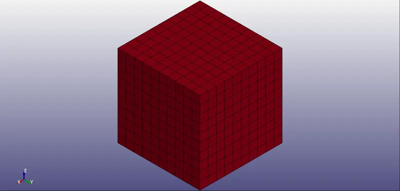
Figure 1.0: 10 x 10 x 10 mm3 comprising of 10 elements in x,y and z respectively.

KEYWORDS:

*MATERIAL

pre-defined in .k file

Material is hyper-elastic

*BOUNDARY

Boundary_spc

• The elements at the bottom (X-Y plane) are constrained in global x,y and z (rotational) and translational z.
• Y and x stability is achieved by constrain the axis of symmetry in translational x, and y.

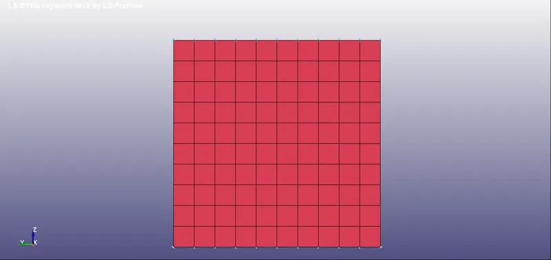
Figure 1.1: Front view for constraints.

Prescribed_motion_set

The elements at top are created under a node set and prescribed motion is assigned as per LCID defined above.

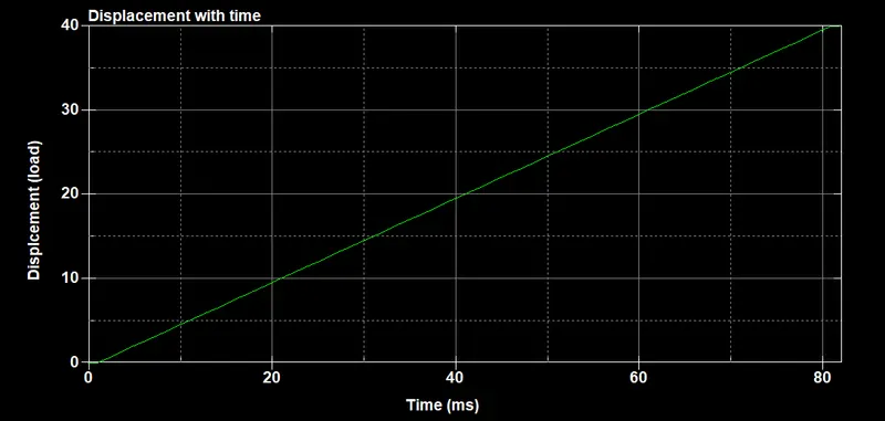
Plot 1.0: Load curve data is loaded from XYdata option imported from XYDATA.csv file.

*SECTION

Solid element section

Case 1-

Element formulation: ELFORM1

Case 2-

Element formulation: ELFORM-1

Case 3-

Element formulation: ELFORM2

Case 4-

Element formulation: ELFORM-2

*DATABASE

ASCII

GLSTAT: DT =0.081

MATSUM: DT =0.081

ELOUT: DT =0.081

BINARY

D3OUT: DT=0.081

EXTENT_BINARY

STRFLG = 1

POST PROCESSING:

Effective V-M stress - and effective strain values are recorded for each load step in all 4 cases.

CASE1: ELFORM = 1

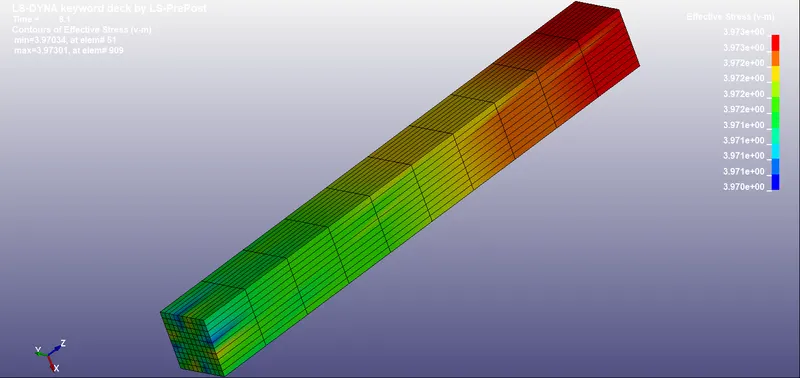
Figure 1.2: Vonimisses stress for Element formulation 1 (At final load step)

For element #661, Stress in z direction and lower Ipt strain in z direction is plotted.

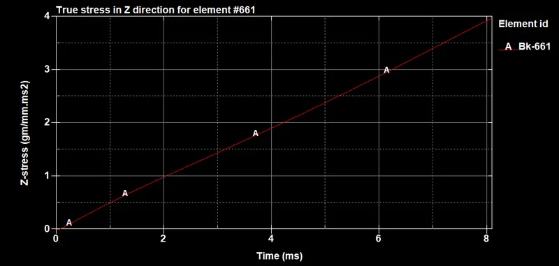
Plot 1.1: Stress induced in z direction for element #661 Vs time.

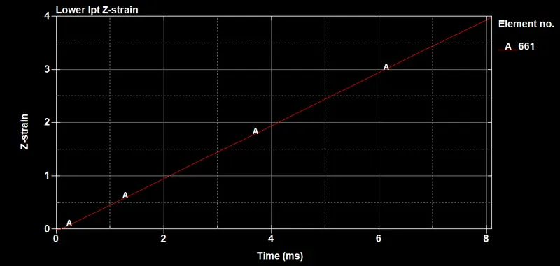
Plot 1.2: Strain induced in z direction for element #661 Vs time

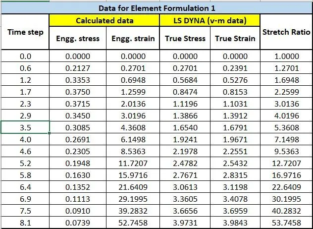
Table 1.1: Data for Stresses/ Strain - Stretch ratio become > 5 at load step 3.5

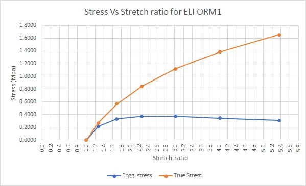
Plot 1.3: Engg stress and True stress Vs Stretch ratio for element formulation 1.

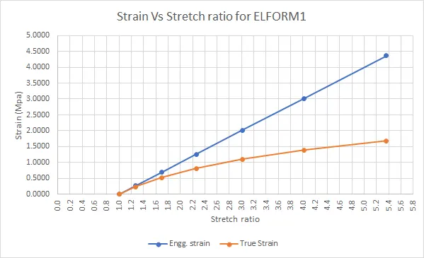
Plot 1.4: Engg strain and True strain Vs Stretch ratio for element formulation 1.

Attachments:

.k file: ELFORM1.k

animation: movie_000_EL1

CASE2: ELFORM = -1

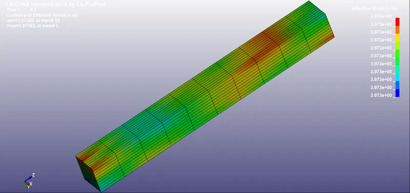
Figure 1.3: Vonimisses stress for Element formulation -1 (At final load step)

For element #661, Stress in z direction and lower Ipt strain in z direction is plotted.

Plot 1.5: Stress induced in z direction for element #661 Vs time.

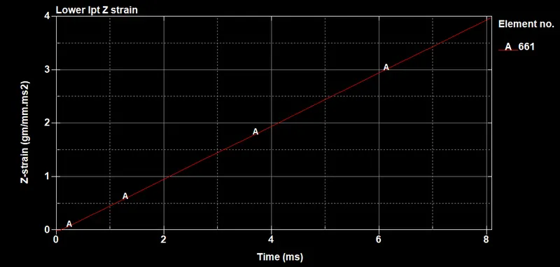
Plot 1.6: Strain induced in z direction for element #661 Vs time

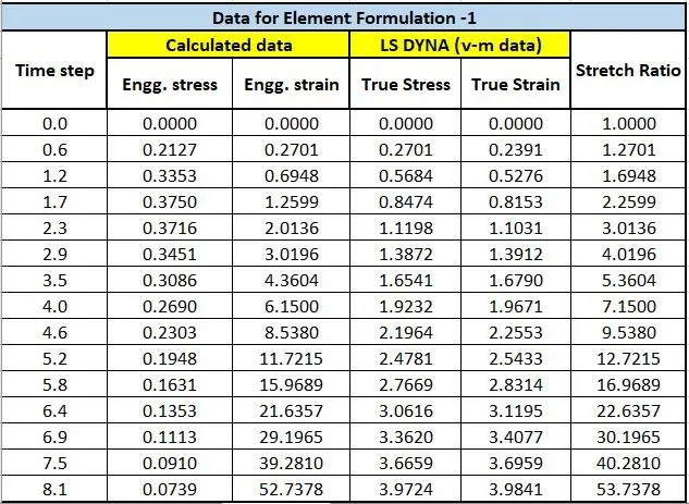
Table 1.2: Data for Stresses/ Strain - Stretch ratio become > 5 at load step 3.5

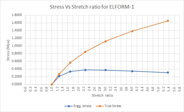
Plot 1.7: Engg stress and True stress Vs Stretch ratio for element formulation -1.

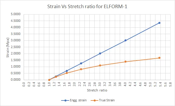
Plot 1.8: Engg strain and True strain Vs Stretch ratio for element formulation -1.

Attachments:

.k file: ELFORMn1.k

animation: movie_000_EL-1

CASE3: ELFORM =2

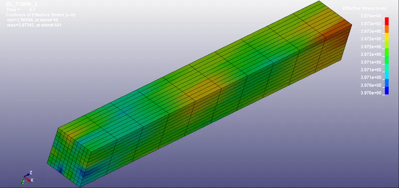
Figure 1.4: Vonimisses stress for Element formulation 2 (At final load step)

For element #661, Stress in z direction and lower Ipt strain in z direction is plotted.

Plot 1.9: Stress induced in z direction for element #661 Vs time.

Plot 1.10: Strain induced in z direction for element #661 Vs time

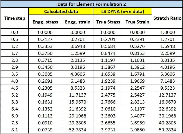
Table 1.3: Data for Stresses/ Strain - Stretch ratio become > 5 at load step 3.5

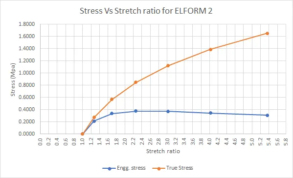
Plot 1.11: Engg stress and True stress Vs Stretch ratio for element formulation 2.

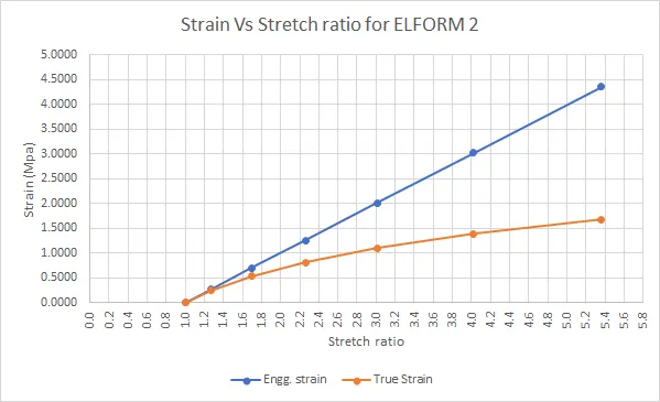
Plot 1.12: Engg strain and True strain Vs Stretch ratio for element formulation 2.

Attachments:

.k file: ELFORM2.k

animation: movie_000_EL2

CASE4: ELFORM = -2

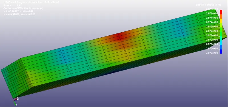
Figure 1.5: Vonimisses stress for Element formulation -2 (At final load step)

For element #661, Stress in z direction and lower Ipt strain in z direction is plotted.

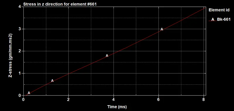
Plot 1.13: Stress induced in z direction for element #661 Vs time.

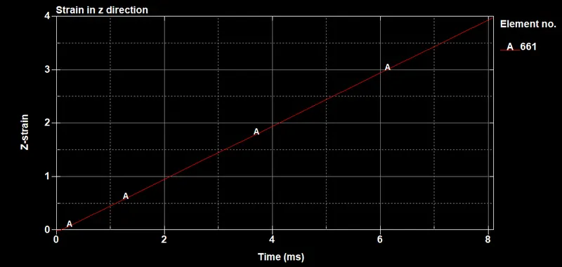
Plot 1.14: Stress induced in z direction for element #661 Vs time.

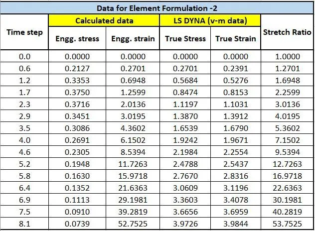
Table 1.4: Data for Stresses/ Strain - Stretch ratio become > 5 at load step 3.5

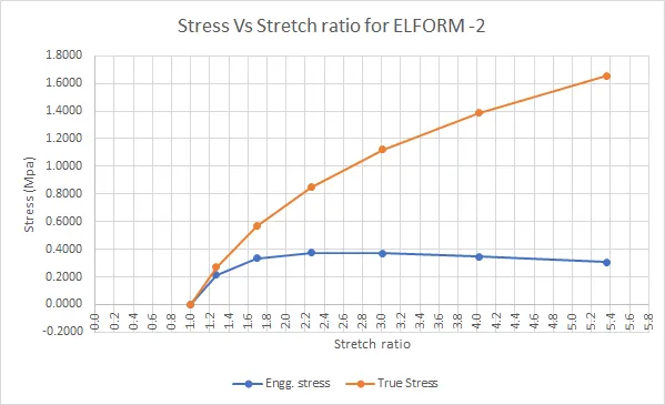
Plot 1.15: Engg stress and True stress Vs Stretch ratio for element formulation -2.

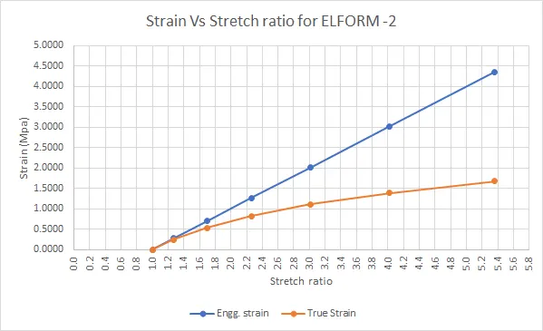
Plot 1.16: Engg strain and True strain Vs Stretch ratio for element formulation -2.

Attachments:

.k file: ELFORMn2.k

animation: movie_000_EL-2

CONCLUSION:

1. Data and plots are almost similar in all four cases.
2. Engineering stress is lower than True stress in all cases.
3. Engineering strain is greater than True strain in all cases.
4. Relationship between stress and stretch ratio is non linear for both stresses.
5. Relationship between engineering strain and stretch ratio represent a straight line(linear). Relationship between true strain and stretch ratio is non linear.
6. The problem is solved using Implicit solver because loading is steady with time. (Not transient). The cube is not in dynamic motion. Strain is uniaxial (z direction) which is achieved using proper SPC boundary conditions.

ATTACHMENTS:

Book1.xlsx contains all data for engineering stresses, true stresses and strains respectively.

.wmv file for 4 formulations has been attached.

keyword file for 4 formulations has been attached.