Week-6 Calculate the Stretch Ratio by comparing the ELFORM (-2,-1,1,2) with Ogden_Material Model.

AIM OF THE PROBLEM

• Create a block of 10mmx10mmx10mm dimension with 10 elements for each direction.
• To use appropriate boundary conditions to simulate uniaxial tensile behaviour of a material.
• Compare the results for the simulation using ELFORM = 1, 2, -1, -2 by plotting Engineering stress versus Stretch Ratio upto Stretch ratio 5.
• Using the proper solver (Implicit or Explicit).

INTRODUCTION

Ogden model was introduced by Ogden in 1972. This material model is a hyperelastic material model used to define the non-linear behaviour of materials like rubber and polymers. This material model is generally used for material showing incompressible, isotropic and non-linear stress-strain behaviour.

A solid cube of rubber material modelled by Ogden material model is simulated for tensile behaviour. Different Element Formulations are used to compare stress versus stretch behaviour.

Which method is best suitable to simulate the given Finite Element model ?

Implicit method is choosen over Explicit method. It is because of the following reasons

• The tensile behaviour of the cube is time-dependent and slow process, where inertial effects are not much important. If it is the case of Explicit method, they are suitable for solving fast process where inertial effects will come into consideration
• This method solves the problem directly by inverting stiffness matrix. Ogden material has a non linear stress-strain behaviour and hence this cannot be solved in one step, but equilibrium iterations would help to solve the problem.

STEPS TO BE FOLLOWED THROUGHOUT THE PROBLEM

Step 1: The given keyword file is opened in LS-PrePost using the option File > Open > LS-Dyna Keyword file. The file consists of only one Material card i.e. *MAT_OGDEN_RUBBER

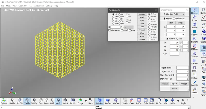
Step 2:- Model Creation: Create a Finite Element Model of a solid block of 10mm x 10mm x 10mm with 10 elements for each direction as shown in the figure. It is created this way. Go to Mesh > ShapeMesher > Entity: Box Solid > Given the required dimensions as shown in the figure > Click on create > Done

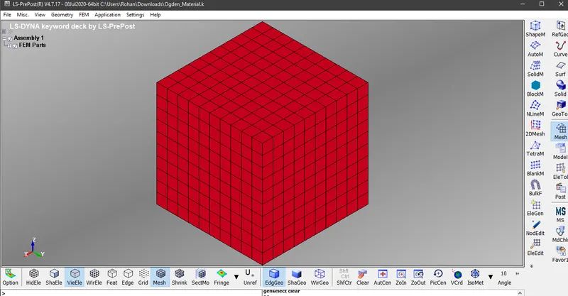
This is how the model exactly looks like in its element mode. It is projected in Isometric view.

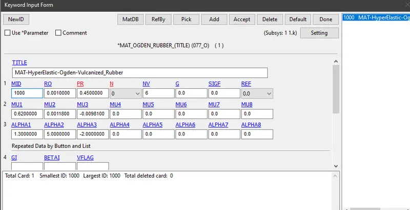
Step 3:- Review the material properties which was given along with keyword file: A separate material card has been created named *MAT_OGDEN_RUBBER which is used to define the non-linear behaviour of materials like rubber and polymers

Note: The unit of µ in the material definition is in MPa and α is a dimensionless quantity

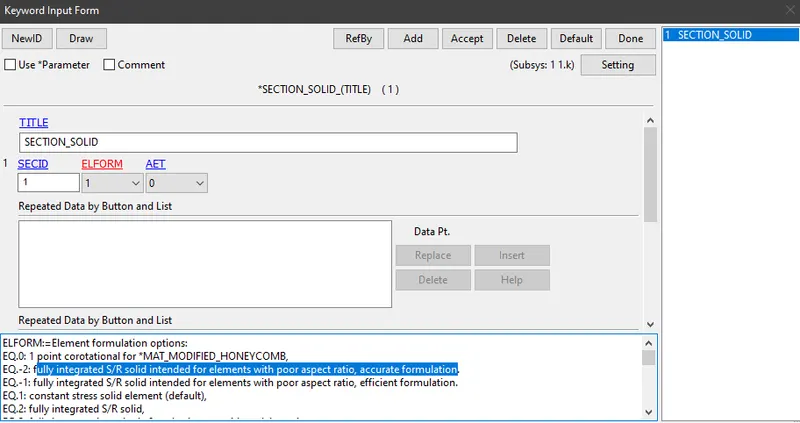
Step 4 :- Create a solid section for Finite Element Model with different Element Formulations: ELFORM 1 refers to Constant stress solid element, ELFORM 2 refers to fully integrated S/R solid, ELFORM -1 refers to fully integrated S/R solid intended for elements with poor aspect ratio, efficient formulation, ELFORM -2 refers to fully integrated S/R solid intended for elements with poor aspect ratio, accurate formulation

Step 5:- Part Definition: The material cards and section cards which have been defined, should be assigned to the respective parts in *PART card

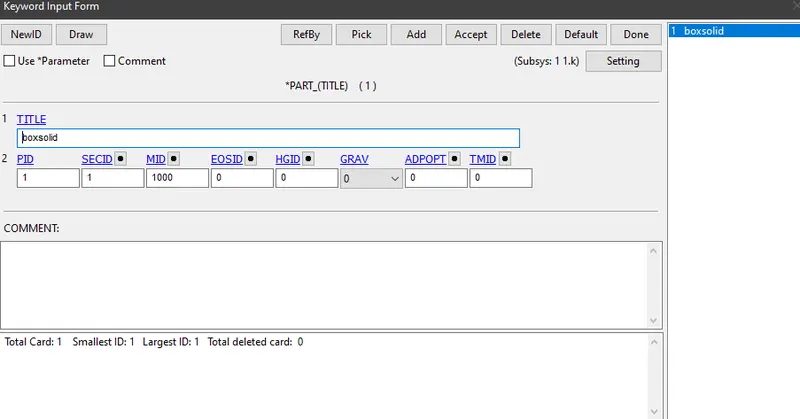
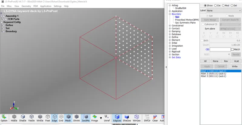
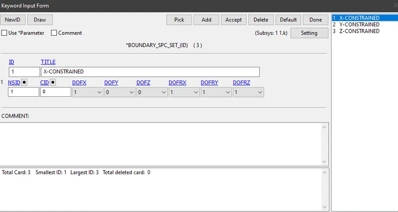
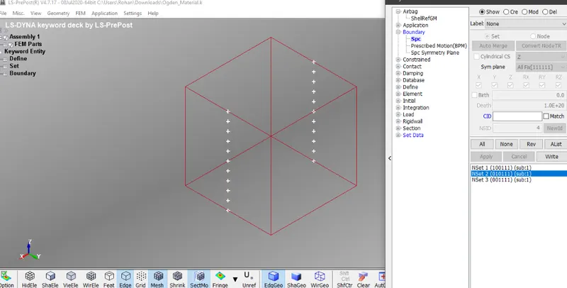
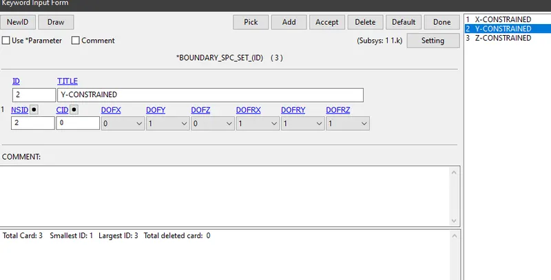
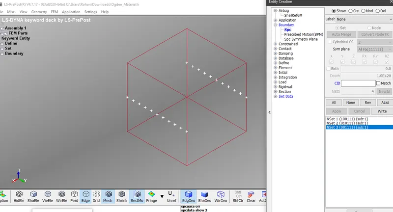
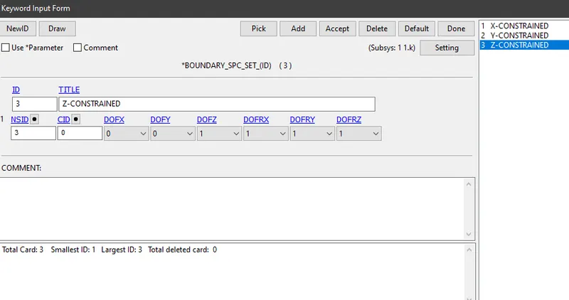
Step 6:- Boundary Conditions: To simulate the tensile behaviour of the model, node at the one end is constrained and node at the other end is prescribed. When a tensile load acts on the cube, it elongates along X-Direction and other face shrinks in small amount. The center nodes of the faces should be constrained, so that they do not move. Three Boundary SPC sets should be created that are translational along X, Y and Z directions.

Case (i): Boundary SPC set when constrained along X-direction

Case (ii): Boundary SPC set when constrained along Y-direction

Case (iii): Boundary SPC set when constrained along Z-direction

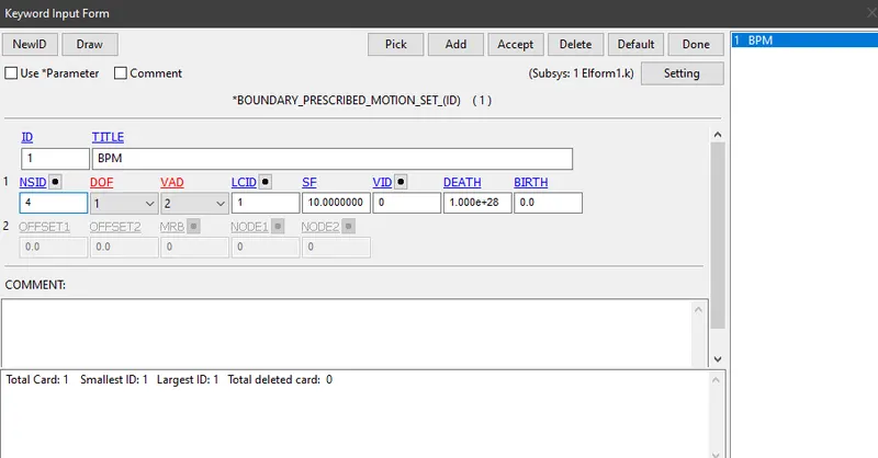
Step 7:- Boundary Prescribed Motion(BPM): To simulate the tensile behaviour, the face opposite to the constrained face along X-direction should be given with displacement and stretch ratio should be taken as 5.

λ = 1 + ε_e , where ε_e= δl / l

λ = 1 + (δl / l)

5 = 1 + (δl / 10)

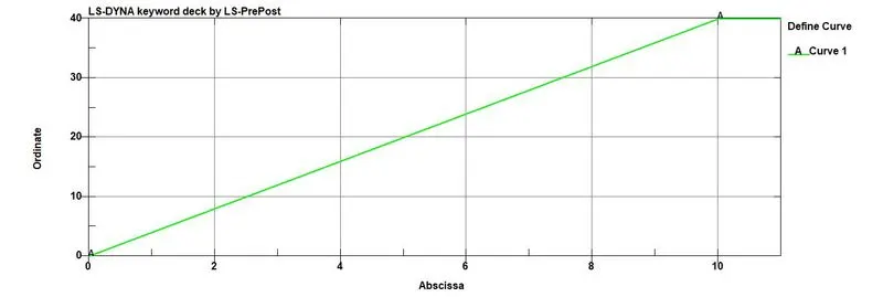
δl = 40 mm

Hence 40 mm is considered to define the load curve

(a) Create a boundary condition for prescribed motion

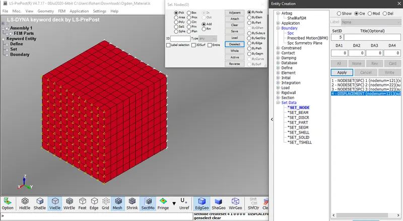
(b) Thus, a load curve has to be defined to allocate it in *Boundary_Prescribed_Motion

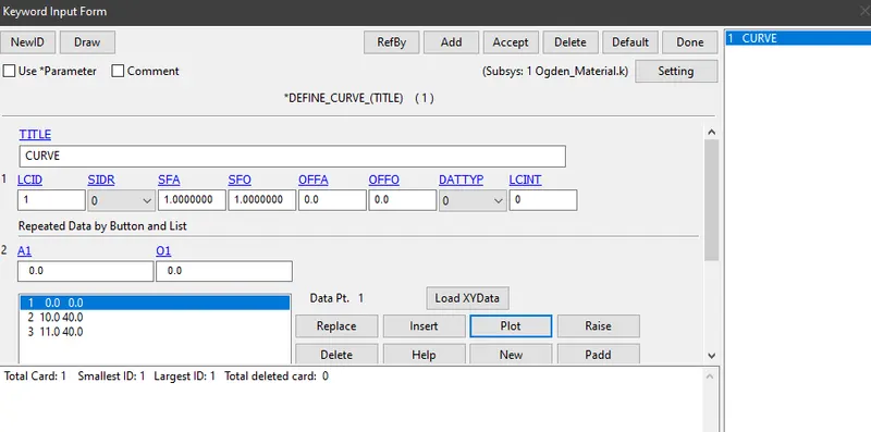
(c) Plot the load using the values of Abscissa and Ordinate

(d) Define the LCID in *BOUNDARY_PRESCRIBED_MOTION_SET

Step 8:- Define Control cards: Some of the important control cards which is used in Implicit analysis are shown below

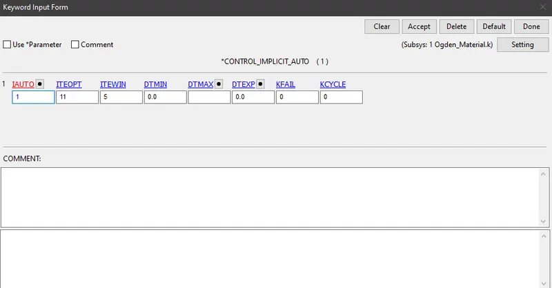
(i) *CONTROL_IMPLICIT_AUTO: It is used for automatic time step control during Implicit analysis. Input value for Automatic time step control flag(IAUTO) is set as 1.

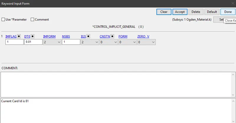
(ii) *CONTROL_IMPLICIT_GENERAL: It is used to activate Implicit analysis and define associated control parameters. This card is required for all types of Implicit analysis. Input value for Implicit/Explicit switching flag(IMFLAG) = 1 and Initial time step size(DTO) for implicit analysis is 0.01

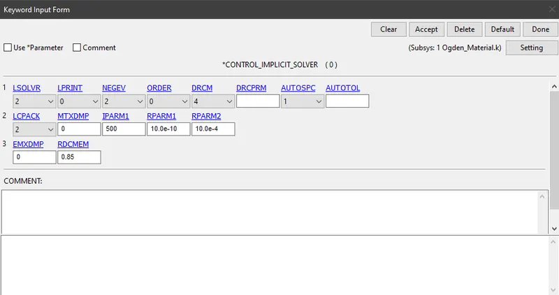
(iii) *CONTROL_IMPLICIT_SOLVER: This keyword is for linear solver parameters and used for implicit calculations.

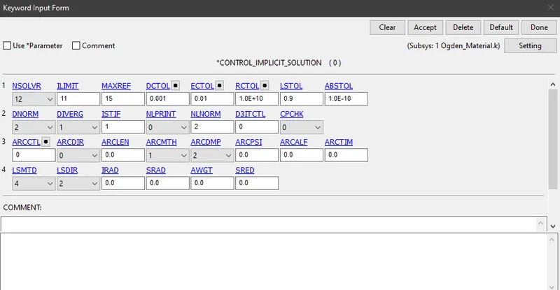
(iv) *CONTROL_IMPLICIT_SOLUTION: This keyword is used to specify whether a linear or non-linear solution is desired. This keyword is for non-linear solver parameters.

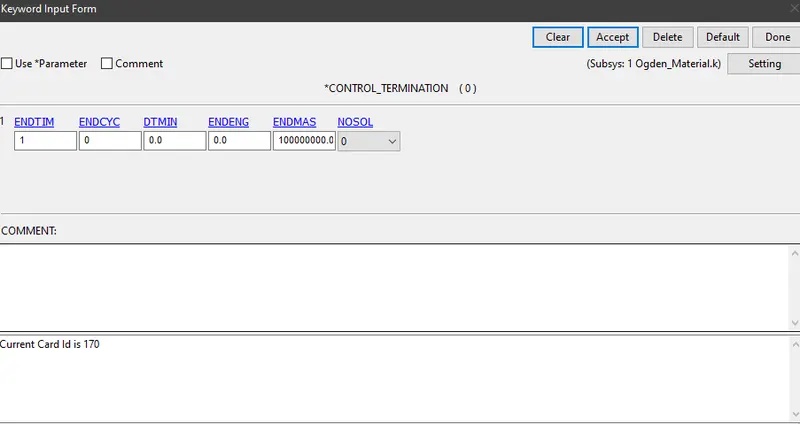
(v) *CONTROL_TERMINATION: It is enabled to specify the end time of the simulation and termination time is set for 1 ms.

Step 9:- Providing necessary conditions for output file

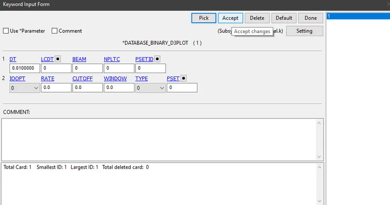
(i) *DATABASE_BINARY_D3PLOT: It is used to get the outputs. Time step should be given as 0.01

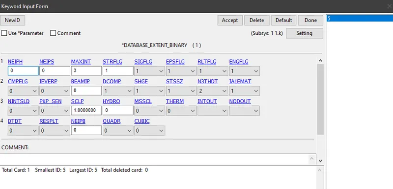
(ii) *DATABASE_EXTENT_BINARY: It is used to compute elastic strain in the model and some of the strain data. STRFLG should be given as 1.

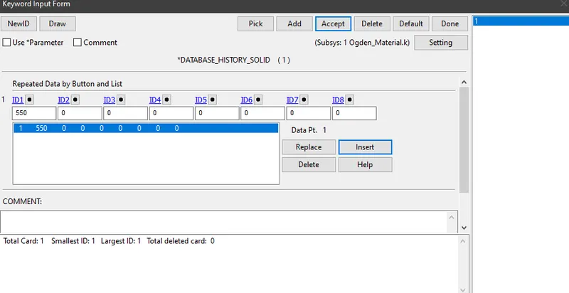
(iii) *DATABASE_HISTORY_SOLID: It is used to compute stress/strain in the model at 550th node.

Step 10:- Keyword check and save the file: Check out for any errors or warnings under keyword check. If there are no errors in the model, save the model using .k extension. (Note: Warnings can be ignored some times)

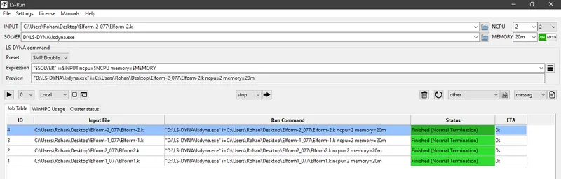
Step 11:- Run the saved keyword file of Element formulation 1 using LS-Run. If it is a Normal termination, post processing is carried out. If it is an error termination, recheck the model.

If it is a normal termination, then change the element formulations to 2, -1 and -2 individually and run the model using LS-Run

I) RESULTS

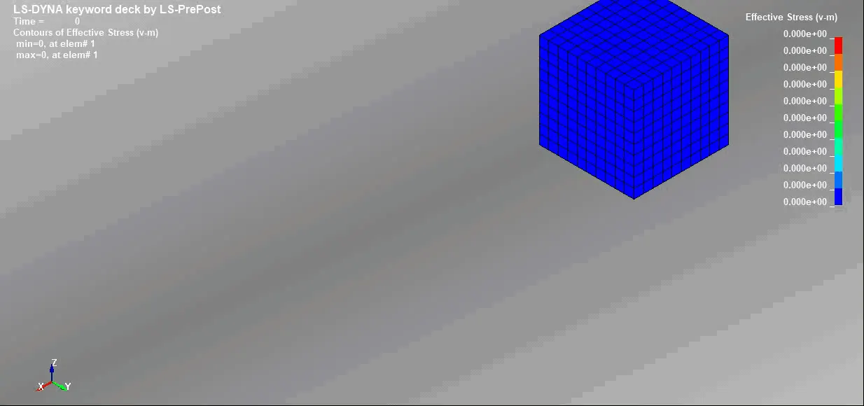
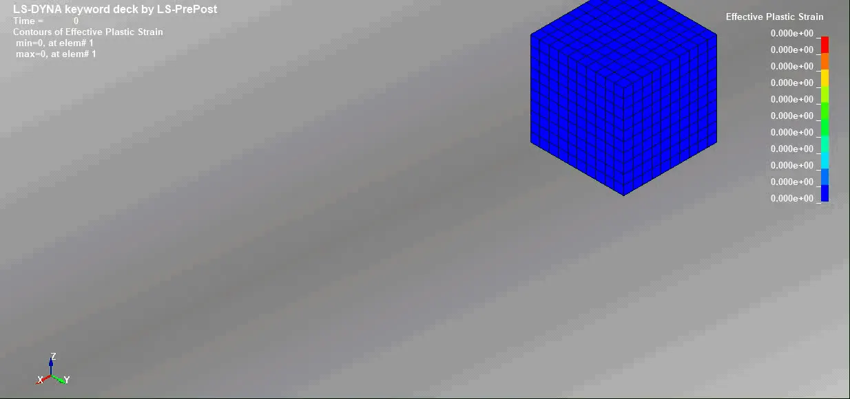
a)Effective stress and Plastic contours when Element Formulation is 1. The maximum value of stress is 3.9 MPa and maximum value of strain is 2.3

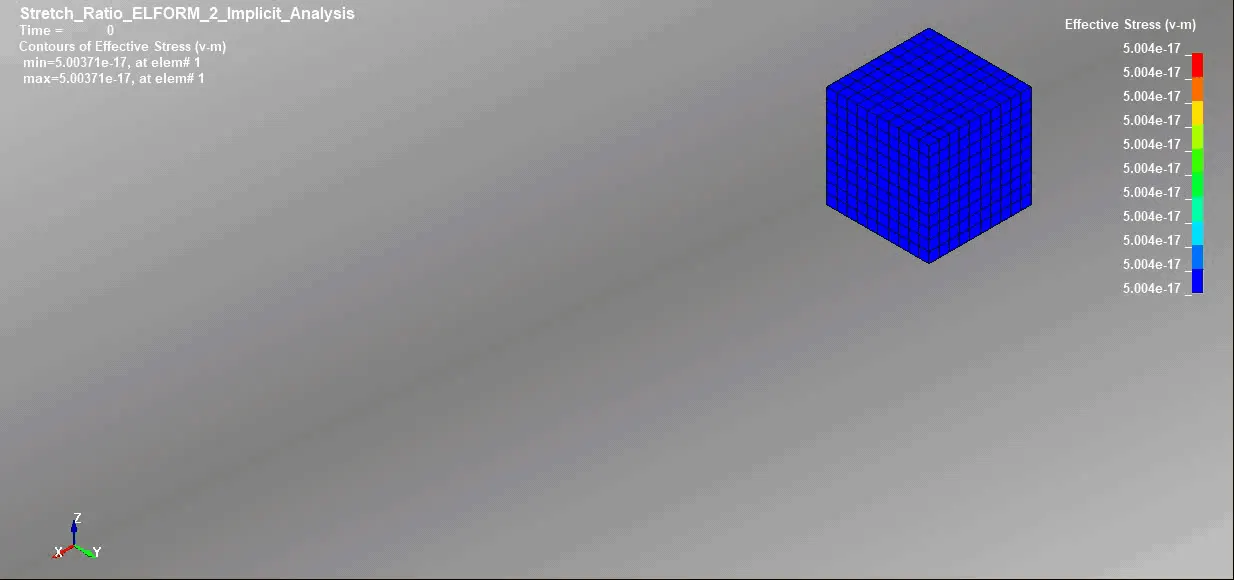
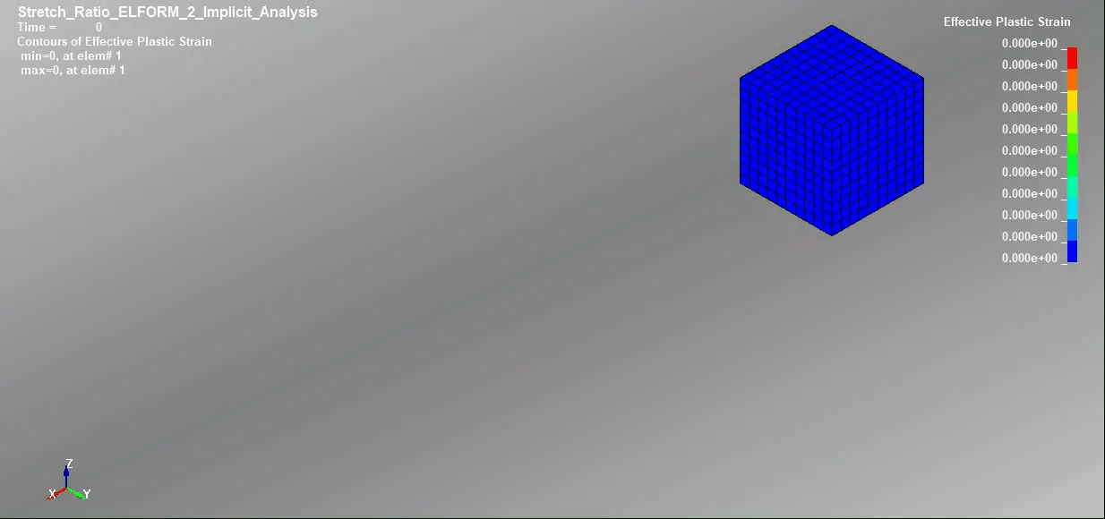
b)Effective stress and Plastic contours when Element Formulation is 2. The maximum value of stress is 3.96 MPa and maximum value of strain is 2.37

c)Effective stress and Plastic contours when Element Formulation is -1. The maximum value of stress is 3.97 MPa and maximum value of strain is 2.37

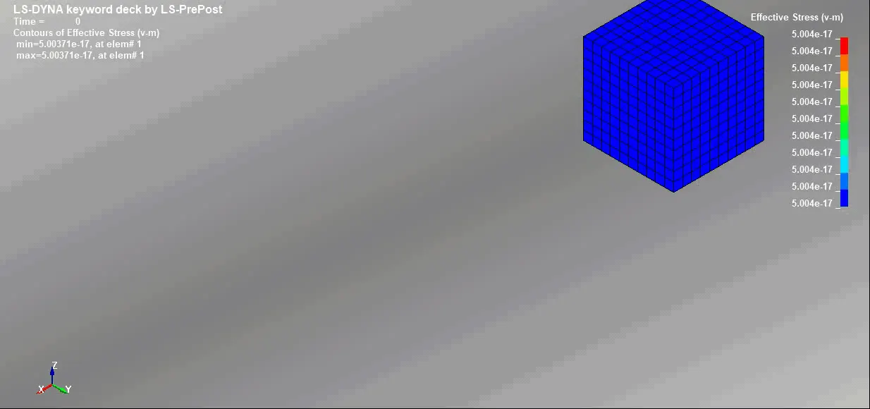
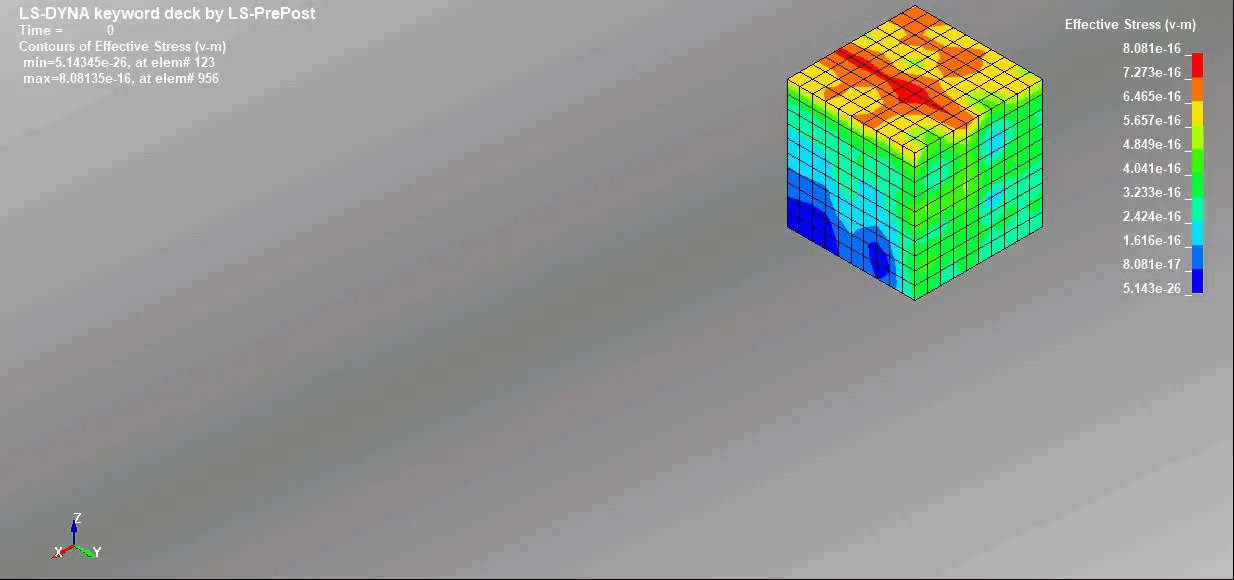
d)Effective stress and Plastic contours when Element Formulation is -2. The maximum value of stress is 3.97 MPa and maximum value of strain is 2.3

(II)Calculation of Engineering stress, Engineering strain and Stretch Ratio

True stress, σ_t = σ_e (1+ ε_e)

Engineering stress, σ_e = σ_t / (1+ ε_e)

True strain, ε_t = ln(1 + ε_e)

Engineering strain, ε_e = e^εt - 1

Stretch Ratio,λ = 1 + ε_e

Conclusion from the graphs plotted: The engineering stress value corresponds to a stretch ratio of 5 is almost 0.8 MPa approximately in four cases. The following are the graphs plotted between Stretch Ratio along X-axis and Engineering Stress along Y-axis

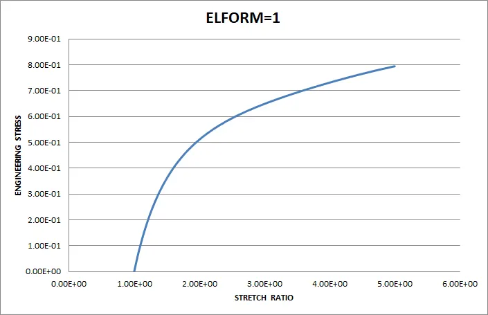
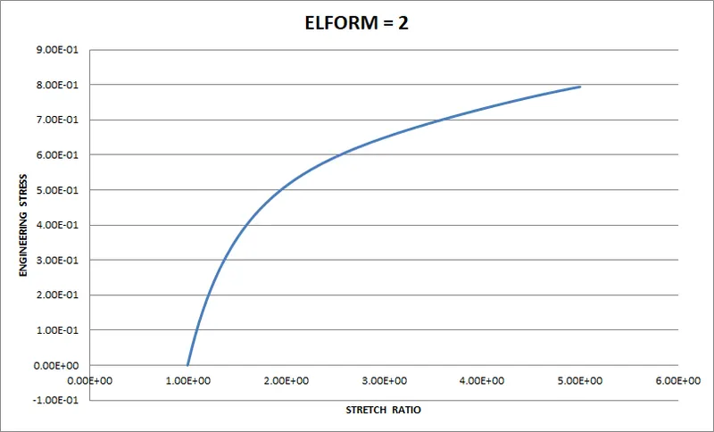
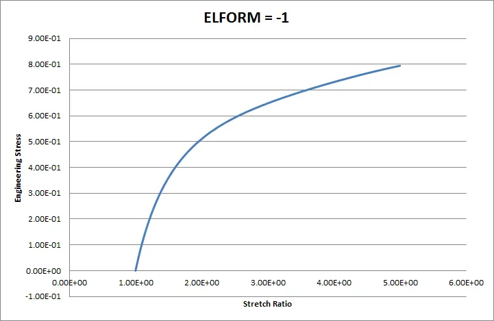
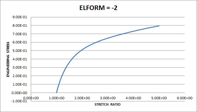
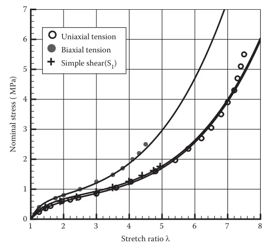
Conclusion from the actual plot given: The actual plot for Nominal stress and Stretch ratio for ogden material is shown in the below graph. In the actual plot, the value of Nominal Stress for a stretch ratio of 5 is 1.8 MPa. But from the simulation results the value of stress is 0.8 MPa for a Stretch ratio of 5. It is observed that the variation of 1MPa stress is occured during simulation for uniaxial tension test of ogden material. It is because of Non-linearity of the material and relatable boundary condition applied for the model.

FINAL CONCLUSION

• The given Finite Element model of solid block was created the help of Ogden material to simulate Uni-axial tension test for different Element Formulations.
• The graphs were plotted between Stretch ratio and Engineering stress.
• The actual graph and graphs obtained from simulation is being compared.
• The Uniaxial tension test was solved using Implicit solver since the analysis is similar to Quasi-Static analysis on a hyperelastic non linear material.

Simulated keyword files can be accessed using the link given below through Google drive

https://drive.google.com/drive/folders/1PqrLGRaDuvrFp1OP8Cwlx2-m79bhrzDO?usp=sharing