Week-6 Calculate the Stretch Ratio by comparing the ELFORM (-2,-1,1,2) with Ogden_Material Model.

Objective:

To Create a block of 10mmx10mmx10mm dimension with 10 elements for each direction and to use the material card attached (Ogden_Material.k) , then simulate using approximate boundary conditions with the element formulation of 1,2,-1,-2 and comparing the results by plotting Engineering stress vs Stretch ratio with appropriate solver (Implicit/Explicit).

Procedure:

Case setup and Execution:

• Open the keyword file Ogden_Material.k in LS PREPOST.
• The file consists only of Ogden material Card

1. Modelling the cube:

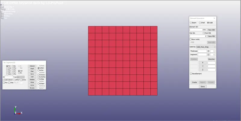
• To model the cube the following steps are followed Mesh `rarr` Shape Mesher `rarr`IN the Shape Mesher Choose Box solid As Entity `rarr` Dimensions as 10*10*10.

Section creation:

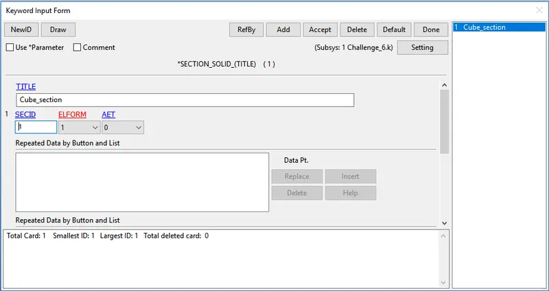
• Shell section is needed to be defined by selecting Keyword manager `rarr`All `rarr`Section `rarr`Solid
• Here the solid selection with element formulation 1 is defined , Similarly we need to define element formulation as 2,-1,-2 for all other cases to solve the problem

Case 1: ELFORM = 1, constant stress solid element.

Case 2: ELFORM = -1, Fully integrated S/R solid intended for elements with poor aspect ratio, efficient formulation.

Case 3: ELFORM = 2, Fully integrated S/R solid

Case 4: ELFORM = -2, Fully integrated S/R solid intended for elements with poor aspect ratio, accurate formulation.

There are four cases which are to be simulated after the boundary condition setup to compare and plotting the results.

Specifying section and materials to their respective part ID's :

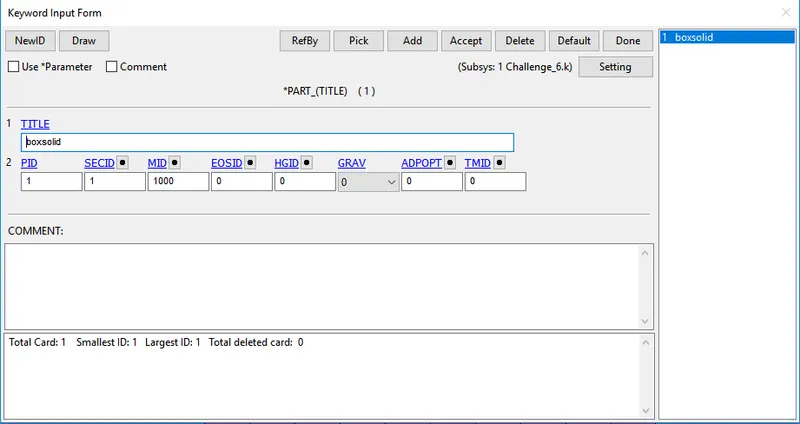
• For creating the part Keyword manager `rarr`model `rarr` part is used , then the respective section and material is assigned to it.

2. Specifying the Boundary conditions:

• Our major aim is to perform uniaxial tensile test on the given model which can be done when one end of the cube is fixed and the other needed to be specified with a prescribed motion set
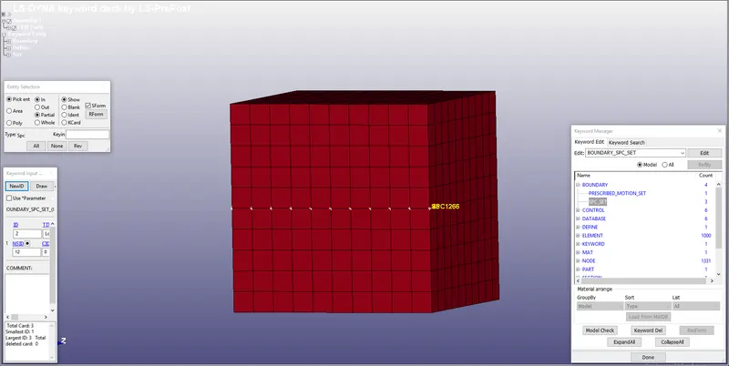
• Hence The Nodes Of One of the Faces Are fixed Using SPC as shown below,
• Create Enitity `rarr`Boundary `rarr`SPC

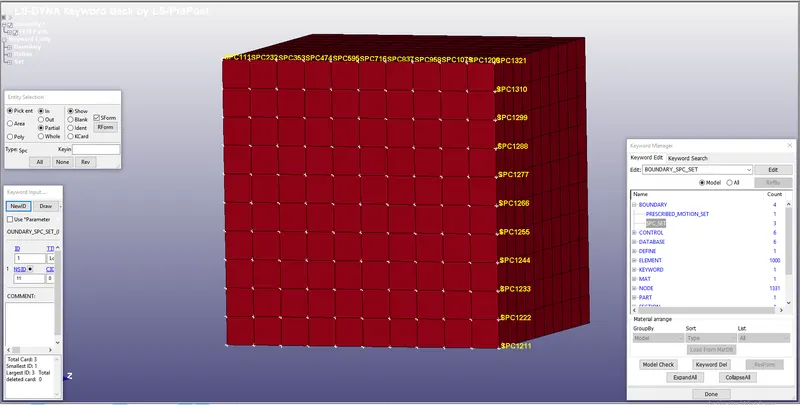
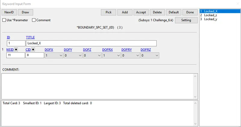
The Nodes in the Middle is selected and Dof's are given According To the Deforming Consideration.

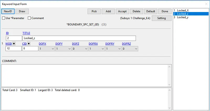
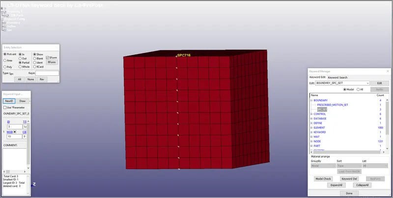
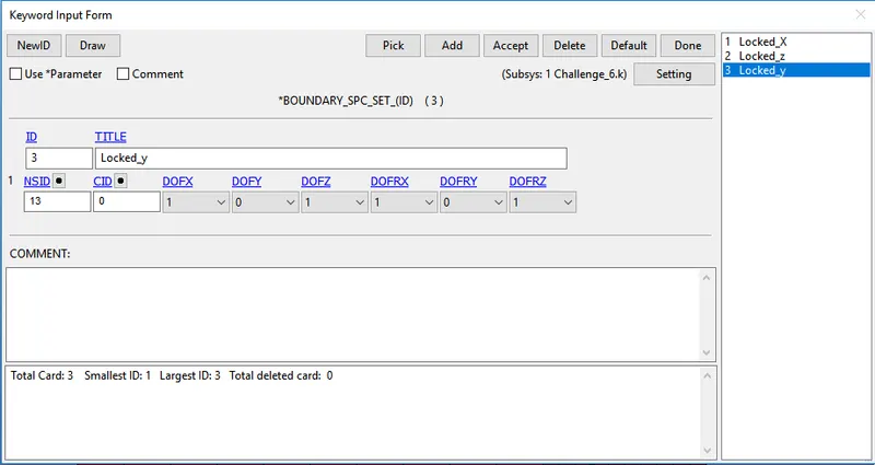
Defining Prescribed motion set:

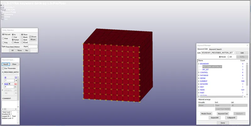
• A set of nodes opposite to the fixed face is selected and named as displacement nodes
• Create Enitity `rarr`Boundary `rarr`Prescribed motion set

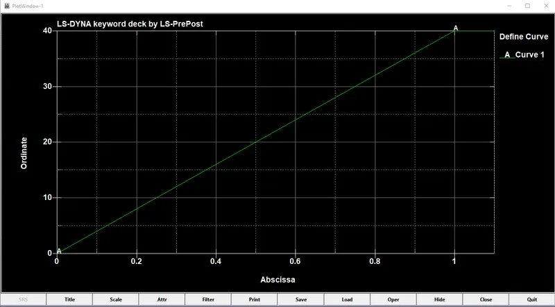
• The Load to be Applied On the Moving face to attain stretch Ratio is calculated

  Stretch ratio l is defined as the ratio between the final length L and the initial length `L_0` of a component i.e. it is equal to (1 + engineering strain)

  `lambda = 1+epsilon_e`

  Engineering Strain `epsilon_e`= `( deltaL)/L`

  `lambda=5,L=10`

  `5=1+(deltaL)/10`

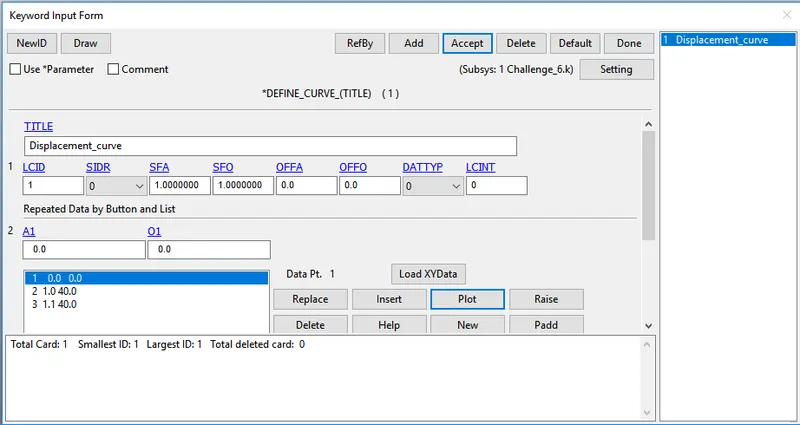
  `deltaL=40mm`

A curve is defined with the Displacement of 40mm

The displacement curve is assigned to the displacement nodes created of Prescribed motion Set

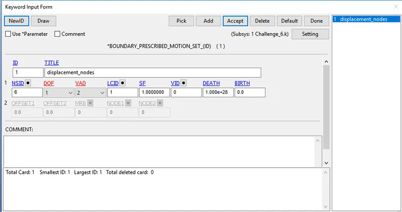
the Material here is Ogden model which is hyperelastic material model that can be used for predicting the nonlinear stress-strain behavior of material such as rubber or polymer. In the Implicit method, displacement loading is recommended rather than Force load to achieve a more stable load. So this Problem is Solved using Implicit.

3. Control Cards:

In LS prepost generally the solver used is Explicit, to perform in Implicit solver the following keywords are needed to be defined to switch from implicit to explicit

i.Keyword manager `rarr`All`rarr` control `rarr` Implicit_Auto

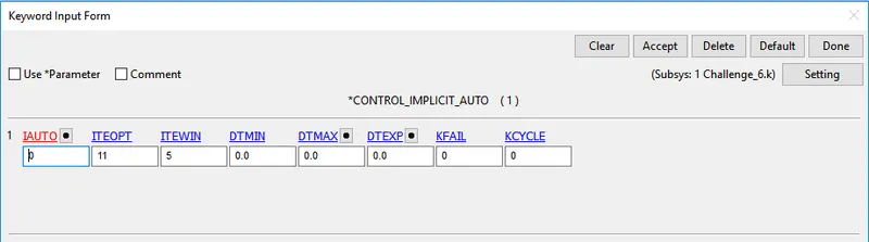
CONTROL_IMPLICIT_AUTO card is used for automatic time step control during implicit analysis. Input value for Automatic time step control flag = IAUTO = 0.

ii.Keyword manager `rarr`All`rarr` control `rarr` Implicit_General

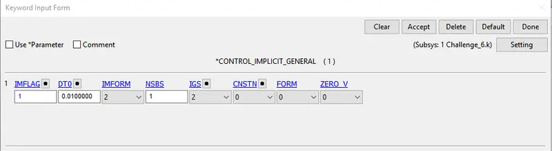
• CONTROL_IMPLICIT_GENERAL card is used to activate implicit analysis and define associated control parameters. This keyword is required for all implicit analyses.
• The input value for IMFLAG=Implicit/Explicit switching flag = 1 (implicit analysis)
• DT0=Initial time step size for implicit analysis = 0.01.

iii.Keyword manager `rarr`All`rarr` control `rarr` Implicit_Solution

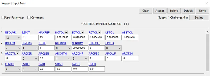
CONTROL_IMPLICIT_SOLUTION card is used to specify whether a linear or nonlinear solution is desired. The default values are set as it is in the card.

iv.Keyword manager `rarr`All`rarr` control `rarr` Implicit_Solver

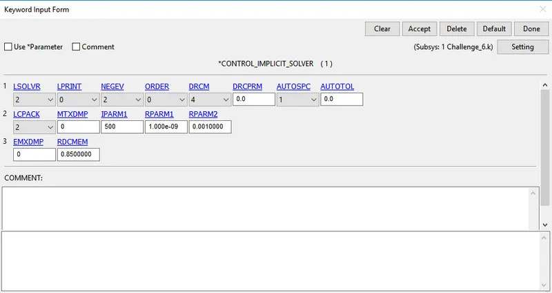
CONTROL_IMPLICIT_SOLVER card is used for implicit calculation.

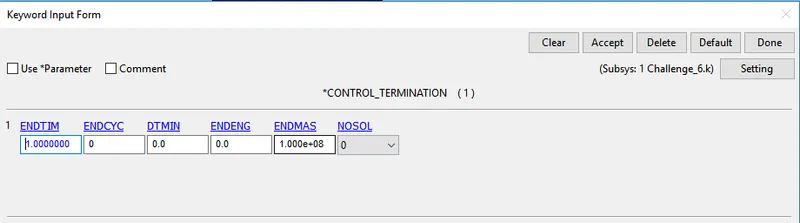
v.Keyword manager `rarr`All`rarr` control `rarr` Termination

Here the termination time is given as 1ms

4. Output request:

Output request:

• Generally output resquest are specified to view the results of the simulation which is done by the following commands
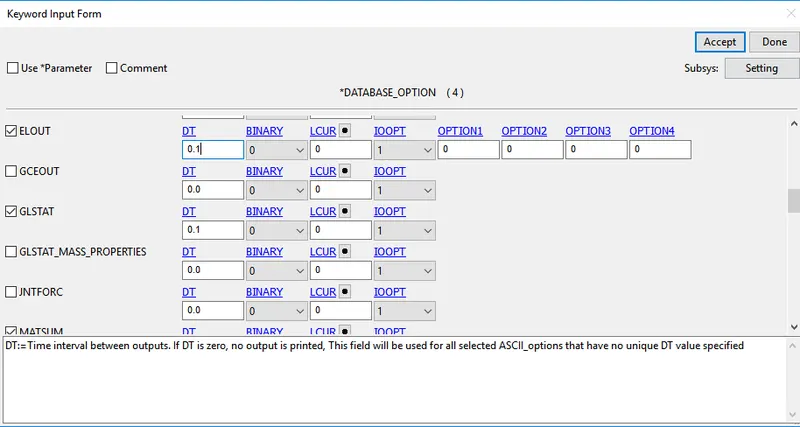
• Keyword manager `rarr`All`rarr` Database`rarr` ASCII_option from which GLSTAT,MATSUM and ELOUT option is selected with DT= 0.01 ms
• GLSTAT is defined with DT=0.01 ms which gives the output of energies such as Internal energies, kinetic energy & other types of energies
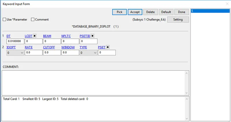
• Keyword Manager `rarr`Database `rarr` Binary D3plot `rarr` DT 0.01, this command prints the output at the end of each 0.01 ms
• Keyword Manager `rarr`Database `rarr` Extent_binary with IMFAG = 1 is given , this will compute the elastic strain in the model

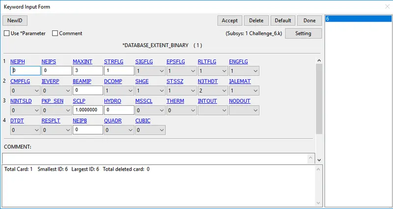
5. Run the simulation

• The keyword is saved in a separate folder and it is opened in Ls-Dyna manager

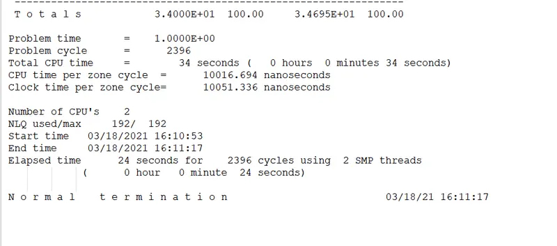
RESULTS:

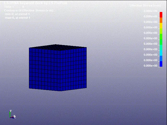
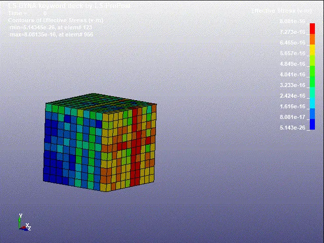
Case i: Element Formulation 1 :

Effective stress:

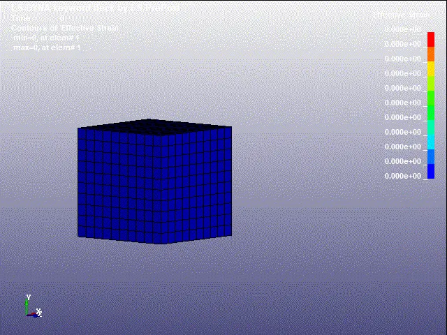
Effective strain:

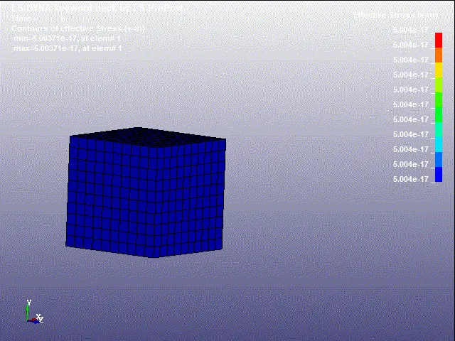
Case ii: Element Formulation -1 :

Effective stress:

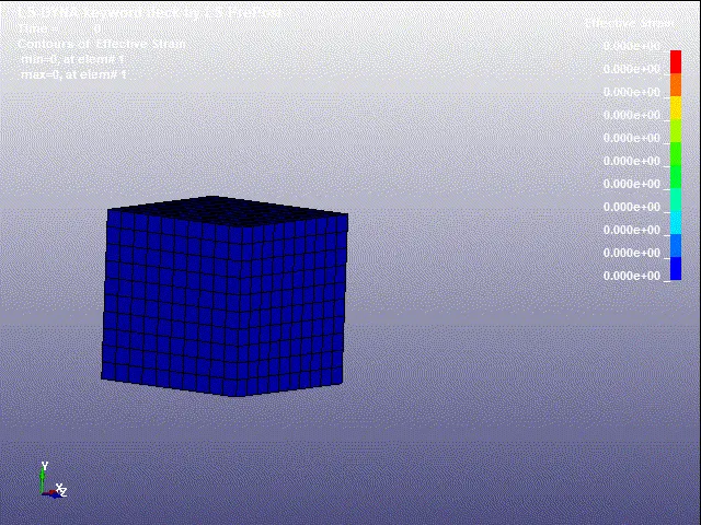
Effective strain:

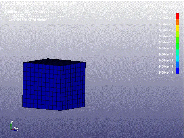
Case iii: Element Formulation 2:

Effective stress:

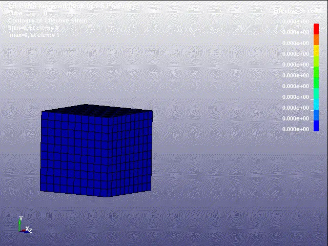
Effective strain:

Case iv: Element Formulation -2:

Effective stress:

Effective strain

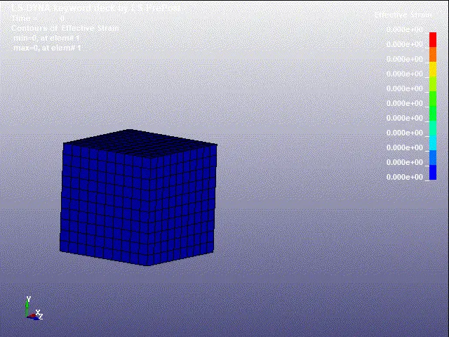
The Value Of strain is equal in all cases where there is a slight change in the Stress value but it's almost the same in all cases.

Calculation of Engineering Stress, Strain and Stretch Ratio:

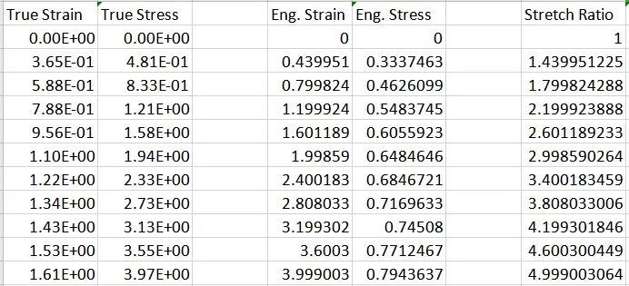
The Output Stress and Strain Obtained From The Post-processing are Noted as True Stress and Strain values,

We know that,

True stress, σt=`σe(1+epsilon_e)`

Engineering stress, σe=`sigma_t/(1+epsilon_e)`

Similarly,

True strain, ϵt=`ln(1+epsilon_e)`

Engineering strain, ϵe=`e^(epsilon_t)-1`

Stretch ratio, λ=`1+epsilon_e`

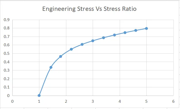
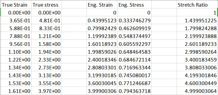
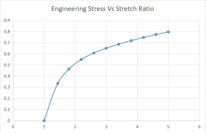
An element is selected as random in the Box and its value of Stress and Strain Are Plotted.

Case i: Element Formulation 1 :

Case ii: Element Formulation -1 :

Case iii: Element Formulation 2:

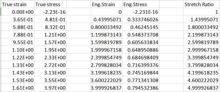
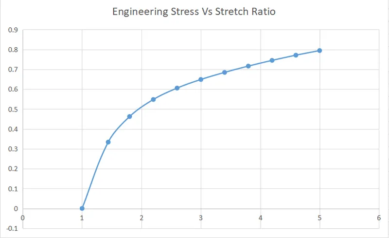
Case iv: Element Formulation -2:

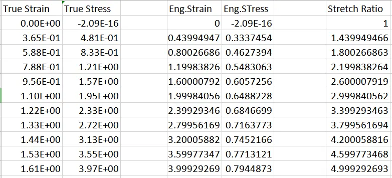
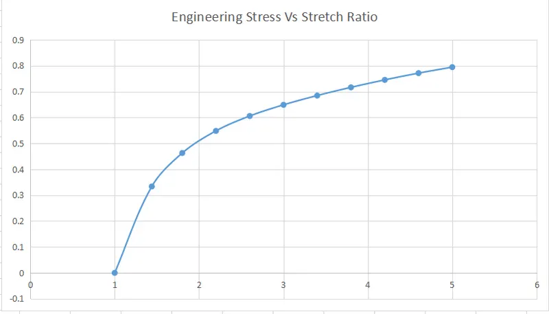
From The Results, we can find that hyperelastic materials exhibit the same Stretch ratios of 5 at 0.8 Mpa

Observation:

ELEMENT FORMULATION	STRESS	STRAIN	STRETCH RATIO
1	3.975	1.476	0.84
-1	3.975	1.476	0.84
2	3.722	1.476	0.84
-2	3.973	1.476	0.84

Since It is a small analysis there is No nodal Displacement occurred and the element formulations didn't exhibit different Properties, whereas working with large elements might show changes in termination time, accuracy based on the element Formulations Used.

Conclusion:

1. Tensile test was simulated for a cube modelled with hexa elements and hyper elastic ogden material model with the test performed for four cases of element formulation of 1.-1,2,-2
2. An implicit method was used to solve this tension problem as the rate of displacement imposed on the model was very low and thus, it was similar to a quasi-static analysis on a hyperelastic elastic non-linear material.
3. The true stress and true strain values are used to find engineering stress and strain values
4. With the Engineering stress and strain values, stretch ratio is calculated and Engineering stress vs Stretch ratio curve is plotted and comapred between all the four cases.