Week-6 Calculate the Stretch Ratio by comparing the ELFORM (-2,-1,1,2) with Ogden_Material Model.

AIM: To calculate the Stretch Ratio by comparing the ELFORM (-2,-1,1,2) with Ogden_Material Model.

THEORY: Ogden material model is a hyperelastic material model used to define the non-linear behaviour of materials like rubber and polymers. This material model is generally used for materials showing incompressible, isotropic and non-linear stress-strain behaviour.

In this study, a solid cube of rubber material modelled by Ogden material model is simulated for tensile behaviour. Different element formulations are used to compare the stress vs stretch behaviour.

Engineering problems can be categorized based on the time scale of physics. Generally, slow processes are time-independent where loads are applied slowly and inertia effects are neglected. Whereas fast processes are time-dependent where inertial effects can not be neglected. The non-linearity increases as the problems become dynamic. Two methods are used to solve these kinds of implicit and explicit method.

IMPLICIT METHOD:

This method is generally used for solving slow processes where inertia effects can be neglected. Here, the problem is solved for the static equilibrium where the sum of the forces is equal to zero. This method solves the problem by inverting the stiffness matrix. We get a solution in one step for simple linear problems but equilibrium iterations are performed within a time-step if the problem is non-linear. The solution is unconditionally stable but at the time steps should be small enough to achieve the convergence for non-linear problems. This method can be used for static and quasi-static problems.

EXPLICIT METHOD:

This method is generally used for solving fast processes where inertial effects are important. The problem is solved for the dynamic equilibrium where the sum of forces is equal to mass time acceleration. This method only increments without any iterations. It is conditionally stable, the time step should be smaller than the critical time step size (Courant-Friedrich-Levy time step). This method is generally used to solve dynamic problems because it handles non-linearities (material, contact and geometrical) with ease.

The tensile behaviour of cube is time-independent and a slow process. The inertial effects are also no important here. So, the implicit method is the best choice for the given problem. The material used for cube is defined by Ogden material model. This has a non-linear stress-strain behaviour and so this cannot be solved in one step but equilibrium iterations would be used to solve this problem.

ELEMENT FORMULATION:

Cube is modelled with a solid element with different element formulations. These are discussed below,

Constant stress solid element (ELFORM 1) is the under-integrated solid element. It needs hourglass control for large deformation problems due to under-integrated formulation. It is efficient, accurate and has low computational cost compared to other solid elements.

Fully integrated S/R solid element (ELFORM 2) is a selective reduced integrated element. The volumetric part of the stiffness matrix has reduced integration formulation which can alleviate volumetric locking issues. But the deviatoric part has fully integrated formulation so, these are susceptible to shear locking.

To resolve this shear locking problem, ELFORM -1 and ELFORM -2 are developed which are similar to ELFORM 2. These solid elements have selective reduced integration formulation which is used to prevent volumetric locking. These solid elements work well for poor aspect ratio as transverse shear energy is not affected by a poor aspect ratio for this formulation. ELFORM -1 has efficient formulation and ELFORM -2 has accurate formulation. ELFORM -2 has higher computational cost than ELFORM -1.

PROCEDURE:

The input keyword file with Ogden material card is given with the problem statement, this keyword file is opened in LS-PrePost.

At first, a solid cube is created in LS-PrePost by using ShapeMesher option in mesh utility. The cube with edge length 100mm is divided into 10 blocks in all three directions. Finally, we get a cube with 1000 solid elements.

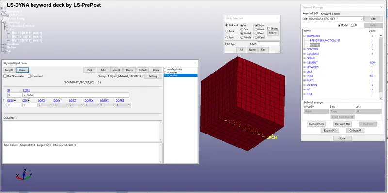
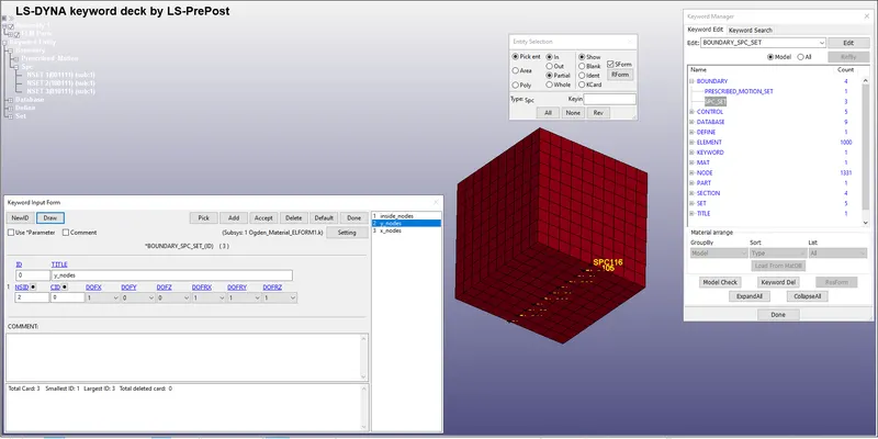
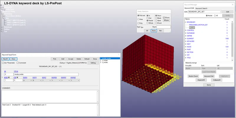
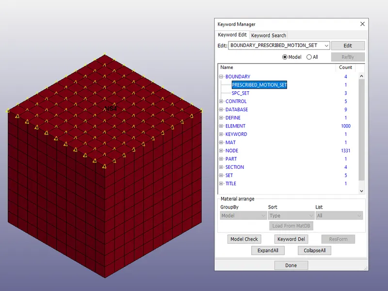
Now to model a tensile behaviour the cube is held from one side and given displacement from the other side. For this single point constraint and prescribed motion boundary conditions are applied through create entity utility. Now, for a tensile test, in reality, the material (cube) will elongate and because of this the cube edges and faces will shrink which are normal to the applied displacement, so these nodes are free to move in those directions and not constrained. Also, the centre node of that face will remain in the same position until the end and will not translate anywhere. Due to the tensile force generated, cube tends to rotate along the axis so even these degree of freedoms are constrained as shown in the following figures.

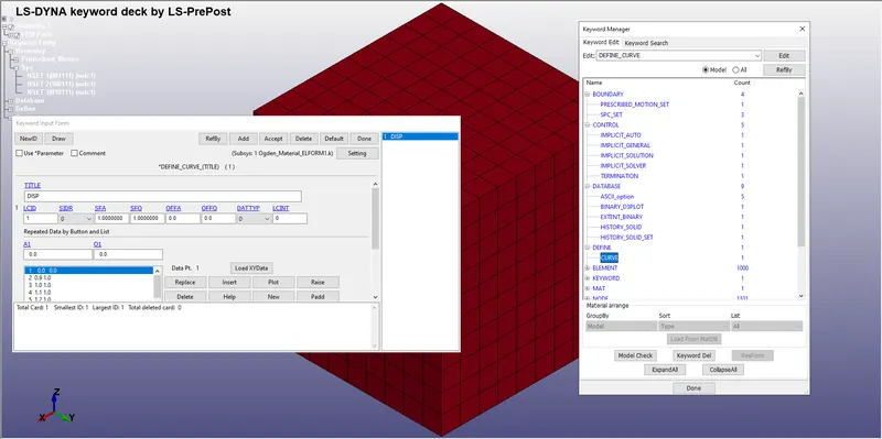
For displacement boundary condition a load curve is defined through which displacement can be applied uniformly and will not be like a step function. If the displacements, loads etc are applied in one step or suddenly, this can generate numerical instabilities. Fig 1.2 shows the load curve used to define displacement behaviour with respect to time.

Displacement is given through *BOUNDARY_PRESCRIBED_MOTION_SET card. The node-set is defined with translational DOF and displacement as a prescribed motion. The cube is given a displacement of 60mm in a positive X direction. The scale factor is set to 60, this will scale the defined load curve which is having 1mm as Ordinate value (displacement). Figure 1.3 shows the card used to defined displacement.

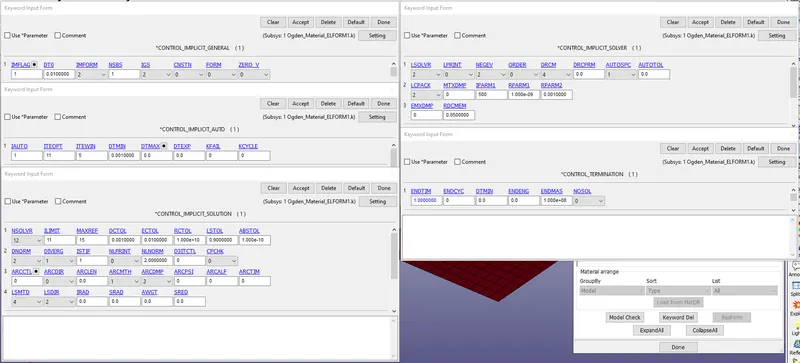
Implicit method is utilized to solve this problem. This method is activated by using *CONTROL_IMPLICIT_GENERAL card. The IMFLAG option is switched to 1 to activate the implicit method. All other options are set to default. Another card *CONTROL_IMPLICIT_AUTO is used which controls the time step size for the problem. Auto-time stepping option is used which will alter the time step size depending upon the number of equilibrium iterations solved within every time step. Optimum equilibrium iterations are set to 50 and iteration window is set to 5. Figure 1.4 and 1.5 shows the control cards used for the implicit method.

The termination time is set to 1ms and if we see fig 1.2, the displacement is also applied uniformly up till 1ms. For post-processing, various database cards are used to extract the results. BINARY_D3PLOT is used to extract the animation data, GLSTAT is used to extract global statistical data. Sometimes the strain data is not extracted after the simulation, so *DATABASE_EXTEND_BINARY card is used which writes the strain tensor to d3plot. STRFLG is set to 1. Figure 1.6 shows the assignment of this particular card.

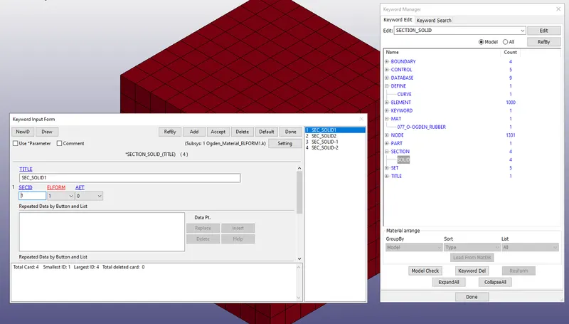
After this, section card is assigned to define the cube with solid elements. In this study, the tensile behaviour of cube is studied with different element formulations. So, element formulation (ELFORM) is set to 1, 2, -1 and -2 according to the problem statement and results are compared for respectively.

For implicit method, matrix inversion takes place this requires a lot of computer memory. So, it is good practice to check the solver output and be sure to run the implicit simulation in-core memory. In-core memory solves the entire stiffness matrix by RAM memory. Whereas out-of-core memory solves a part of the matrix in RAM memory and transfers the data continuously to a disk memory, this takes more time. The memory in LS-DYNA is given in M words. A memory of 10000000 is defined for this setup to run the analysis in-core memory.

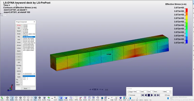
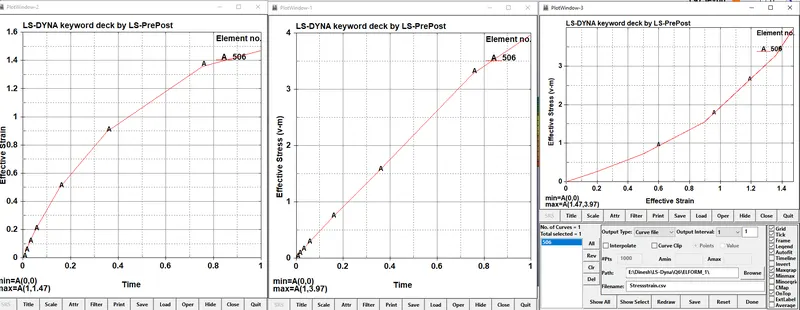
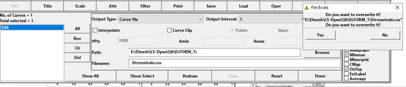
The stress-strain data which is extracted from the analysis is true stress-strain data. But the experimental data given in the problem statement is engineering stress-strain data. So the extracted true stress-strain data should be converted to engineering stress-strain data. This can be done through the following equations:

`εunderset(true)()=ln(1+εunderset(eng)())...................................1`

`σunderset(true)()=σunderset(eng)()⋅(1+εunderset(eng)()).................... (2)`

`εunderset(true)()` = True strain

`εunderset(eng)()` = Engineering strain

`σunderset(true)()`= True stress

`σunderset(eng)()` = Engineering stress

Stretch ratio(𝞴) is the ratio of final length to the original length of the component. The engineering strain is further converted to stretch ratio by the following relation,

`stretch ratio = λ= 1+εunderset(eng)()...................(3)`

RESULTS:

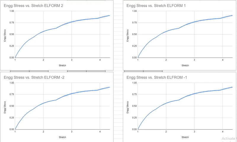
From the above nominal stress vs stretch ratio plots, it can be seen that all the element formulation show similar behaviour. The reduced integrated element formulation (ELFORM 1) takes the least computational time followed by EFLORM 2 which is selectively reduced formulation. EFORM -2 has higher computational cost than ELFORM -1, this is due to a difference in the formulation of strain interpolation matrix.

CONCLUSION:

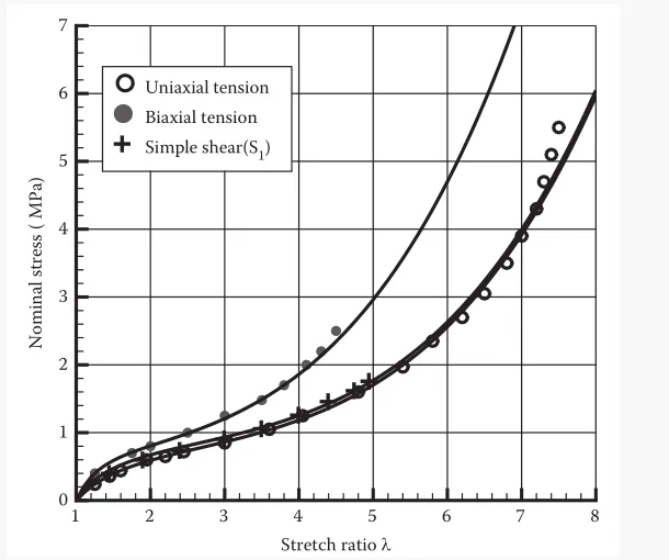
Stretch ratio vs nominal stress data is calculated and plotted for each element formulation. The simulated curves show similar behaviour to the experimental data.

***NOTE:The computational time needed for this cube tensile test simulation is very low. But, the difference due to different element formulation can be noticed for big problems and low aspect ratio geometries.