Week 2 Railwheel and Track

ANSWER

Objective:

1. To perform a static structural analysis on the Rail Wheel and Track.
2. To compare the Total Deformation, Equivalent stress, and the life under different loads/Situation (Multiply the bearing load by 5 times and compare the results with the load of 100000 N)
3. To Implement a User-defined result and calculate the Total Deformation from this result. Also to compare this result with inbuilt result by ANSYS for a load of 100000 N.

Step 1: Engineering Data

• For this analysis we will be using Structural steel as material which can be selected from engineering data under the general material section. It is also added as default material to the drop down list inside material assignment inside the Model.

Step 2: Geometry

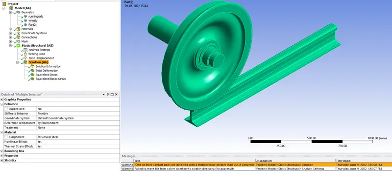
• Right click on geometry and Import the Skill_Lync_Railwheel_Track.x_t extension file
• Rename the Static Structural tab as Rail Wheel Track.
• Update the Static Structural tab and proceed to model.

Step 3: Model

• Open Model and under geometry assign name to geometries.

Step 4: Connections

• Select both the contacts, right click and rename them based on definition.
• Flip the contact and Target.
• Contacts:- Define the contact and Target faces as frictional type and assign a frictional coefficient of 0.3
• Change the Shaft and wheel contact to Frictionless

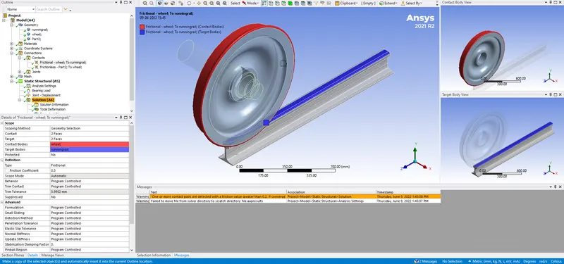
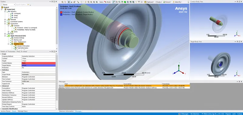
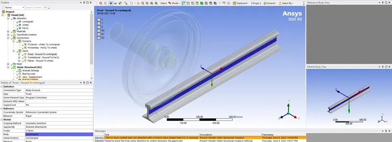
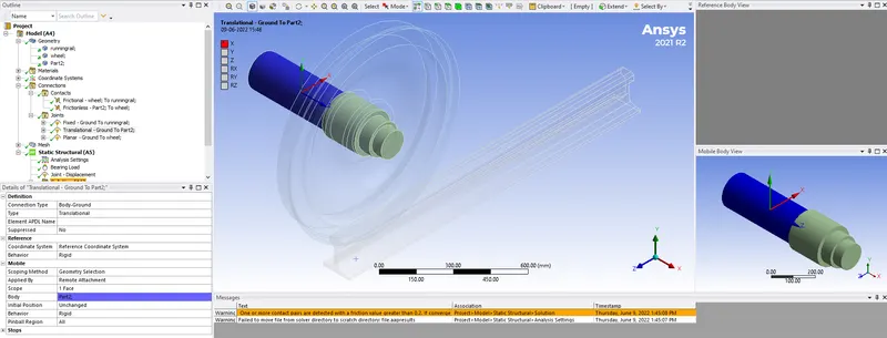
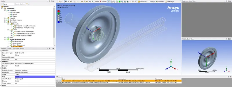
To define the joints for this particular simulation, we have translational motion with rotation along the track. We also need to make sure the wheel stays in one plane. So we need to provide translation joint and planar joints to the wheel. Apart from that we need to provide fixed support which fixes track in place.

• Joint:- Select side face of rail track and assign fixed support joint with Body-to-ground as connection type.
• Select the Shaft surface and assign translational joint to it. Check for the axis of motion and assign the proper axis in that direction.
• Select the face of the wheel and assign planar joint to the wheel.

Select the inner faces of gear geometry to scope and define the type of joint as revolute for both gears.

Step 5: Mesh

• The default mesh is coarse. Assign default element size as 35mm
• Select the three faces in contact which are areas of interest for analysis. Provide face mesh sizing with element size value as 35mm.

Step 6: Setup

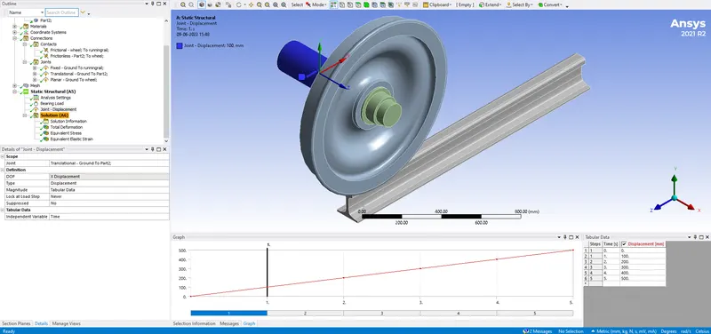
• In analysis settings we are going to simulate this case by moving the wheel 500 mm distance with 100 mm distance in each step..
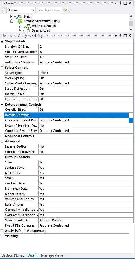
• Enter 5 as the number of steps and select all the steps simultaneously and switch on the large deflection in solver controls.
• Turn on auto time stepping and define as program controlled and solver type as Direct.
• Change all the parameters from output controls to yes.
• Switch on the Force converge in NonLinear Controls
• From Step 2-5 Turn on auto time stepping, define by time, Carry over the time step, with min time as 1e-3 and max time step be 0.1, switch on the force convergence.
• Right click on static structural and insert joint load and assign scope to the joint as translational, with type as displacement and insert magnitude in tabular data with increments of 100mm

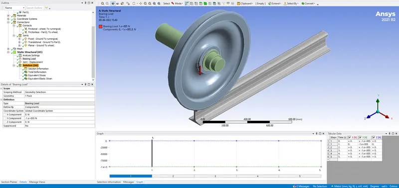
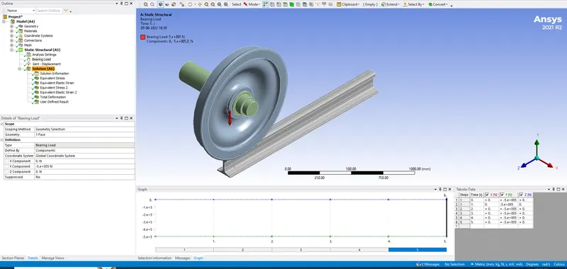
Apart from the translational load, other loads acting upon the wheel are the bearing load, that is load imposed by the carriage will be transferred through the shaft to the wheel through bearing.

• So you can hide the shaft body and insert a bearing load (100000N) on the surface at the hole geometry in the wheel. Define value by components in required direction of motion.

Step 6: Solution

• Insert results for Equivalent Strain distribution, Equivalent Stress distribution, Total Deformation for each geometry in focus to observe the values and data.

Results with Simulation:

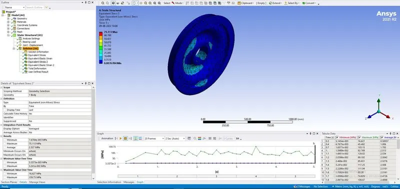
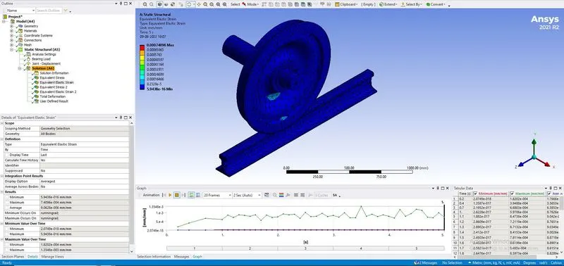
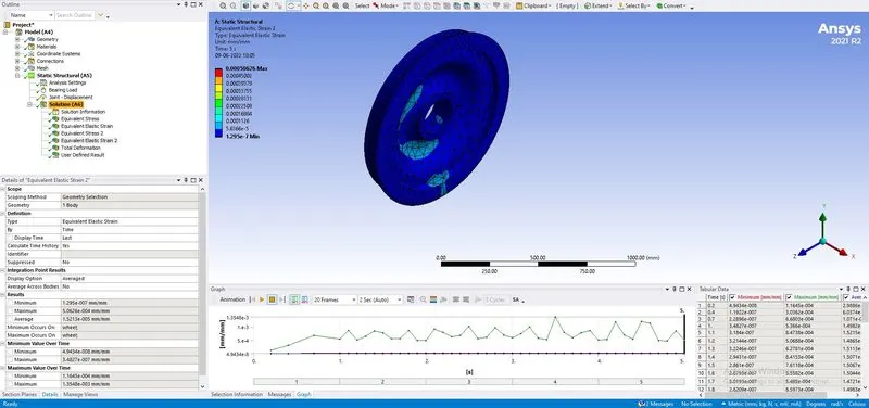
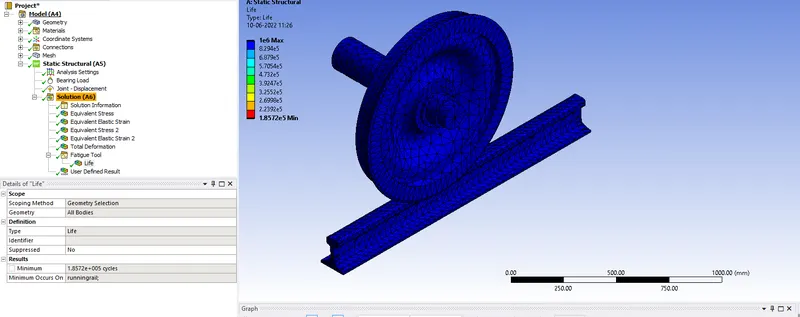
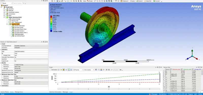
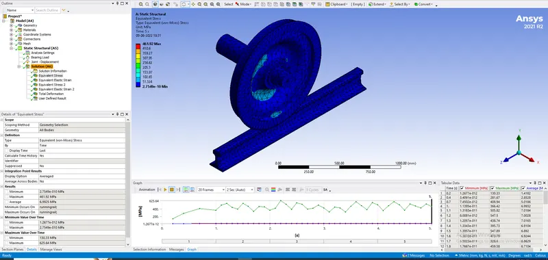
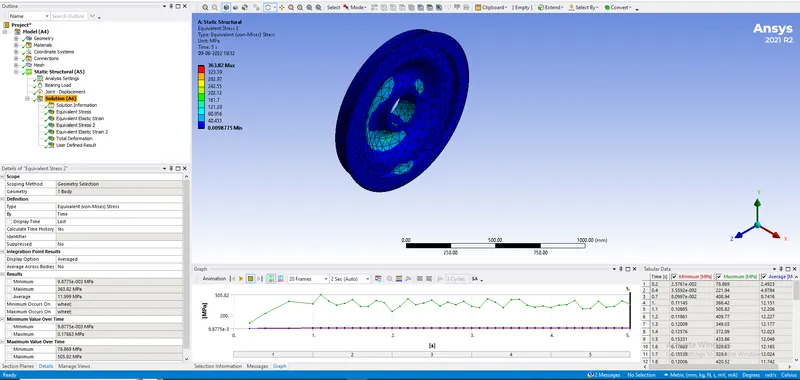
Case 1 Results: Equivalent Strain distribution, Equivalent Stress distribution, Total Deformation.

For 100000N Bearing Load

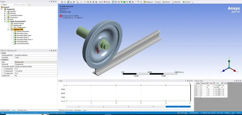
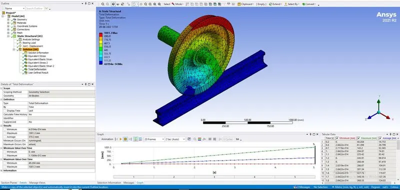
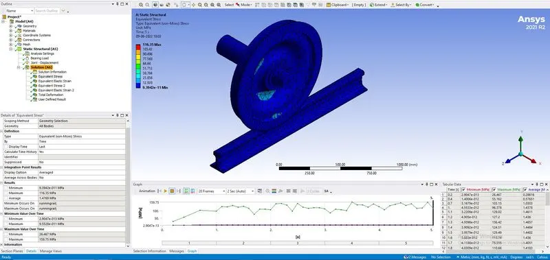
For 500000N Bearing Load

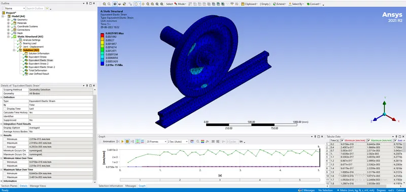
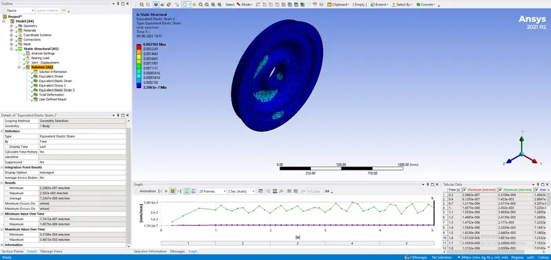
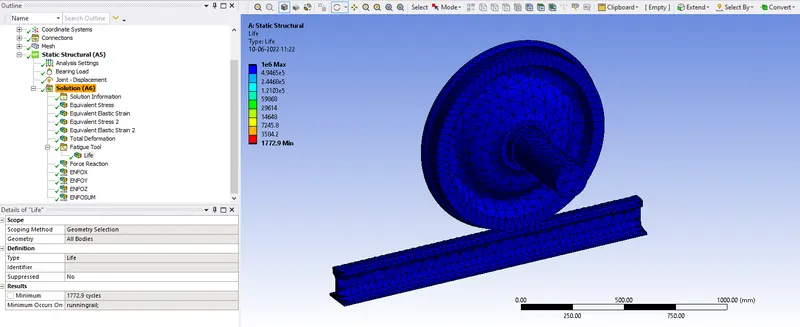
Case 1 Results and Comparison:

Case #	Bearing Load	Total Deformation	Equivalent Strain	Equivalent Stress	Life
Units	N	mm	mm/mm	Mpa	cycles
Original	100000	1001.3	0.00074096	116.35	1e6
1	500000	1001.4	0.00291850	461.92	1e6

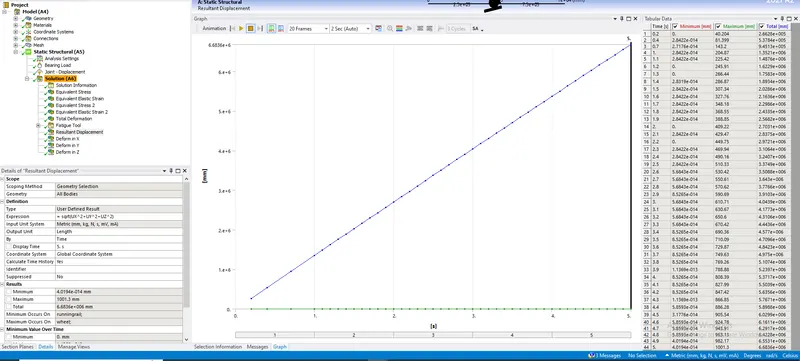
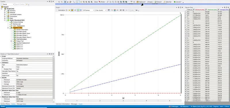
Case 2 Results: User Defined Result and Total Deformation calculation.

User defined result:

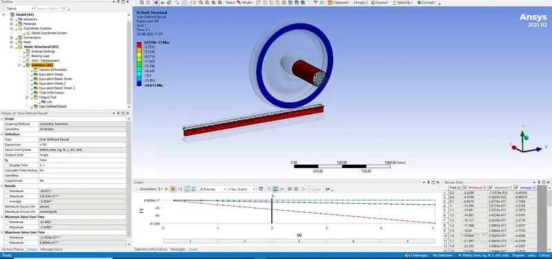
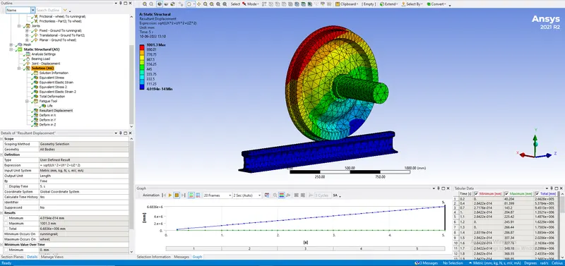
Total Defromation= U Resultant = Sqrt[\(40)Power[UX,2]+Power[UY,2]+Power[UZ,2]\(41)] = 1001.3mm.

User Defined:

Inbuilt Case:

Conclusion:

The results obtained from case 1 show that by increasing the bearing load 5 times, the equivalent stresses developed are 116.53 Mpa nad 461.93 Mpa, i.e increased by almost 4 times. Althoung the fatigue life cycles remain the same for both cases the equivalent strain is 3.93 times the original case. We dont notice a significant change in Total deformation i.e 1001.3 mm and 1001.4 mm for loads of 100KN and 500KN respectively.

Case 2: Results from Inbuilt case are same as User defined results obtained from simulation i.e. 1001.3mm deformation.