Week 2 Bevel Gear Challenge

ANSWER

Objective:

1. To understand Grid Dependency and its uses.
2. To Perform a grid dependency test for the Bevel gear simulation for different mesh sizes
3. To obtain results for Von-Mises stress, Equivalent elastic strain, and Total Deformation using specified mesh sizes.

Grid Dependency Test:

We often face a situation where we have to decide whether the mesh quality is good enough to obtain an accurate solution. A mesh is considered to have higher quality if a more accurate solution is calculated more quickly. Accuracy and speed are in tension. The dilemma here is- decreasing the mesh size always increases the accuracy but also increases computational cost. But, accuracy depends on both discretization error and solution error.

For discretization error, a given mesh is a discrete approximation of the space, and so can only provide an approximate solution, even when equations are solved exactly. For solution error, for Partial Differential Equations’ many iterations over the entire mesh are required. The calculation is terminated early, before the equations are solved exactly. So the choice of mesh element type affects both discretization and solution error.

The overall number of elements as well as the shape of individual elements affect accuracy. The speed of each iteration grows (linearly) with the number of elements, and the number of iterations needed depends on the local solution value and gradient compared to the shape and size of local elements.

If the solution is constant, a coarse mesh may yield an accurate solution; nevertheless, the precision is dependent on the problem instance. In locations where the solution gradients are high, one can refine the mesh selectively, increasing fidelity. Accuracy, including interpolated values within an element, depends on the element type and shape.

Each iteration reduces the error between the calculated and true solution. A faster rate of convergence means smaller error with fewer iterations. A mesh of inferior quality may leave out important features such as the boundary layer for fluid flow. The discretization error will be large and the rate of convergence will be impaired; the solution may not converge at all.

A solution is considered grid-independent if the discretization and solution error are small enough given sufficient iterations. A mesh convergence study consists of refining elements and comparing the refined solutions to the coarse solutions. It determines how many elements are required in a model to ensure that the results of an analysis are not affected by changing the size of the mesh. This test can be carried out by parameterising mesh size and comparing the result value to verify mesh grid dependency. If further refinement or other changes do not significantly change the solution, the mesh is an "Independent Grid."

Procedure:

Step 1: Engineering Data

• For this analysis we will be using Structural steel as material which can be selected from engineering data under the general material section. It is also added as default material to the drop down list inside material assignment inside the Model.

Step 2: Geometry

• Right click on geometry and Import the Skill_Lync_Bevel_Gear.IGS extension file
• Rename the Static Structural tab as Bevel Gear.
• We will be editing the geometry and removing the unnecessary portion/areas of geometry to reduce the redundant calculations and focus on interest areas i.e. stress developed in the tooth area of gears.
• Select the face, and draw a circle with its center coinciding with that of Gear and Pinion with dimension slightly less than that of coinciding geometry.
• Use the pull option to drag the circle and remove the unwanted portion of the model.
• Update the Static Structural tab and proceed to model.

Step 3: Model

• Open Model and under geometry assign name to geometries. Rename smaller gear as “Pinion” and larger gear as “Gear”.

Step 4: Connections

• Contacts:- Reselect all the faces of the Pinion and Gear (16 for Pinion and 24 for Gear) and properly define the contact and Target faces.
• Change the Type of contact to Frictional and Behavior to symmetric.
• Use augmented Lagrange in advanced formulation methods. This is used to avoid the effect of friction on gears and avoid its movement from its location. It increases the stiffness and avoids unnecessary chartering of models.
• Change the interface treatment to adjust to touch under Geometric modification tab

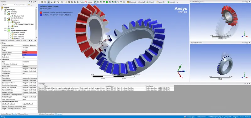
• Joints:- Insert Joint and specify the connection as Body to Ground
• Select the inner faces of gear geometry to scope and define the type of joint as revolute for both gears.

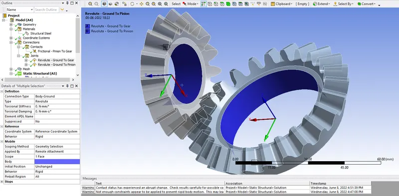
Step 5: Mesh

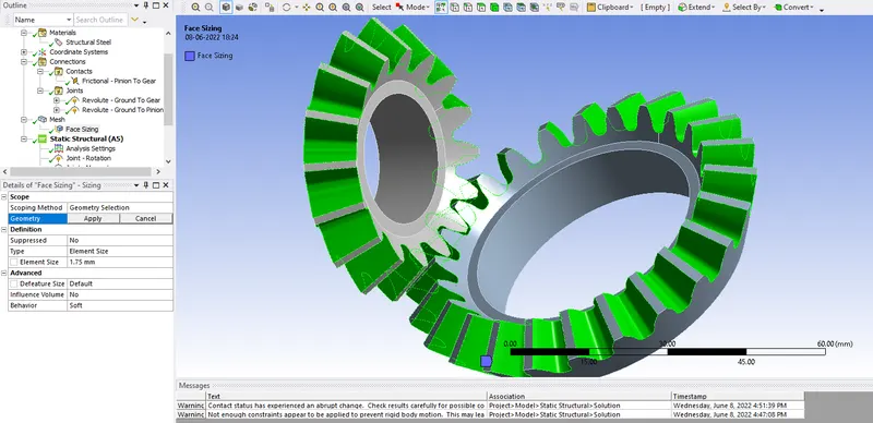
• The default mesh is coarse because of the uniform profile under the gear and this results in convergence issues. To prevent this we use face sizing. Right click on mesh and insert sizing. Select the 40 faces of the tooth across both the Gear and pinion to scope the geometry.
• Within the Mesh option inside the Details of Mesh under default option you can specify Element size and see if the mesh quality is as per required standards.

Case setup and Execution:

Step 5: Setup

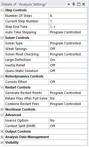
• In analysis settings we are going to divide it in six steps and look at the stresses and forces developed during 120 deg rotation of gear with 20 deg increments.
• Enter 6 as the number of steps and select all the steps simultaneously and switch on the large deflection in solver controls.
• Turn on auto time stepping and define by time
• Put the initial time step as 0.2, minimum time step be 0.1, and maximum step time be 1.
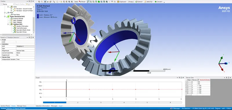
• Right click on static structural and insert joint load and assign scope to the joint and define its type by rotation.
• Assign tabular data for rotation angle for one gear and tabular data with moment values for other gear in the opposite direction of first gear. Tabular increments of 20 deg for rotation and other by moment -Tabular all 100 N-mm values.

Step 6: Solution

• Observe results for Equivalent Strain, distributionEquivalent Stress distribution, Total Deformation to observe the values and data.

Results with Simulation:

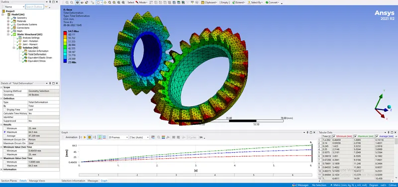
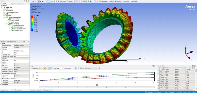
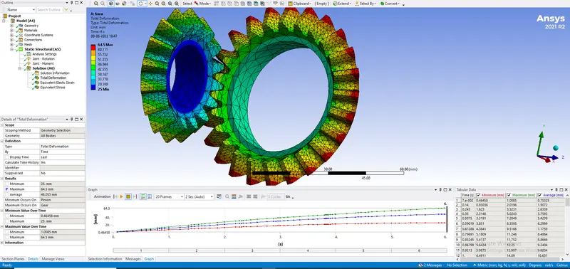
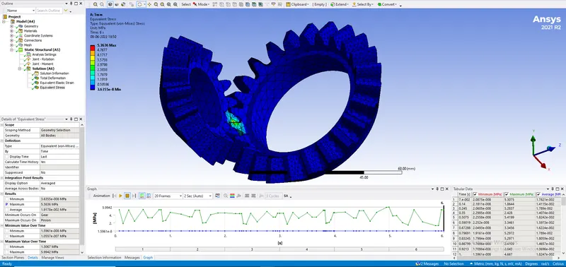
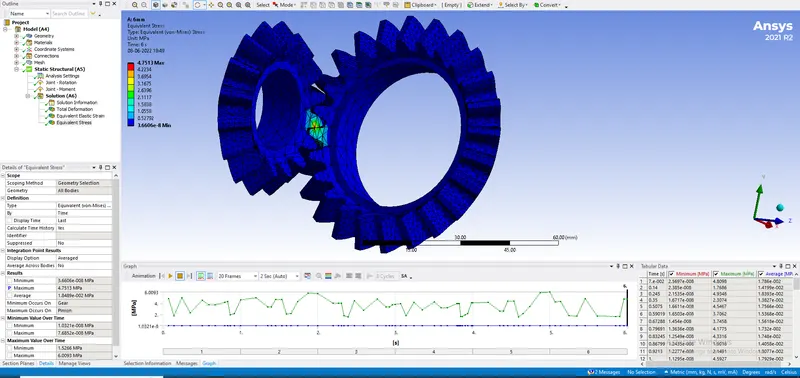
Case #	Mesh Element Size	Face Sizing Element Size	Total Deformation (Max Value over time)	Total Deformation Avg	Equivalent Elastic Strain (Max Value over time)	Equivalent Stress (Max value over time)
Units	mm	mm	mm	mm	mm/mm	MPa
1	4	1.75	64.5	47.209	3.7032e-005	6.1049
2	5	1.75	64.5	47.739	3.5558e-005	5.9942
3	6	1.75	64.5	48.053	3.5232e-005	6.0093
4	7	1.75	64.5	48.140	4.1711e-005	7.1878

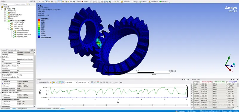
Equivalent stress results for the Setup:

Total Deformation results for the Setup:

Equivalent Elastic strain results for the Setup:

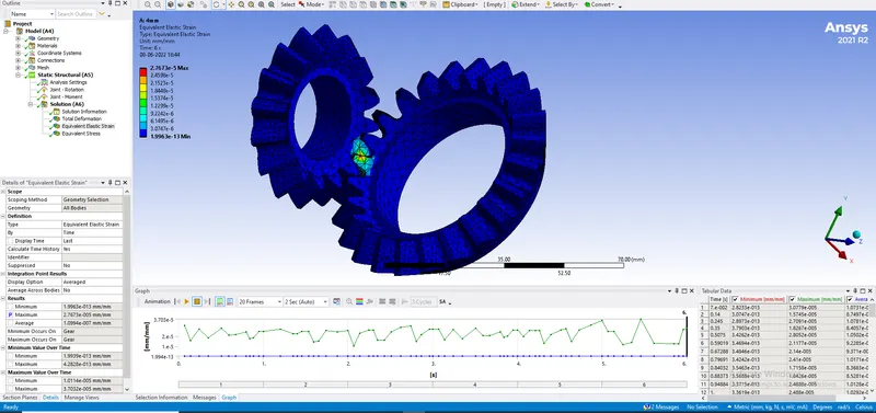
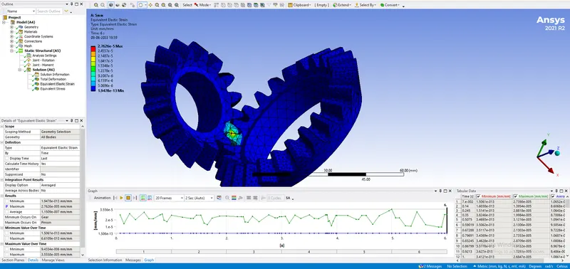
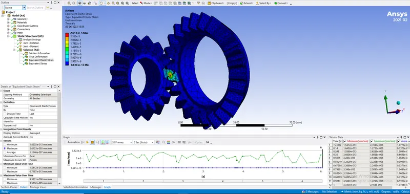
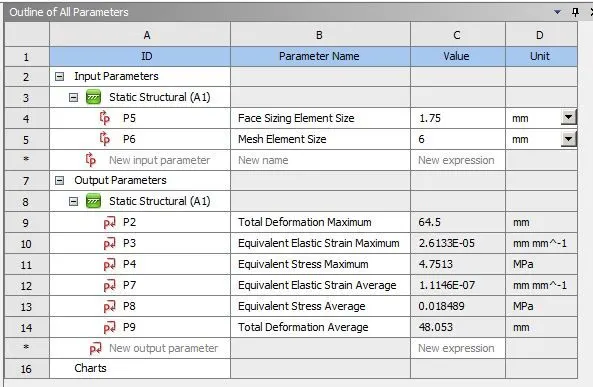
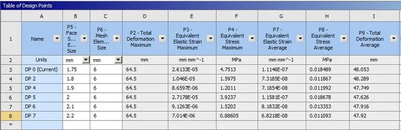
Conclusion: By parameterising mesh size and comparing the result value to verify mesh grid dependency we see that the total deformation for all three cases remains the same as 64.5mm. We find the Equivalent Stress values for 7mm, 6mm, 5mm, 4mm are 7.1878 Mpa, 6.0093 Mpa, 5.9942 Mpa, 6.1049 Mpa respectively. Corresponding Total deformation values are 48.140 mm, 48.053, 47.739 mm, 47.209 mm respectively. Here we notice extending simulations beyond 5mm mesh size does not further affect the results and will only increase calculation time and required computational power. Thus 5 mm mesh size can be considered as optimum and at this point we can say that mesh is grid independent.

Simulation Files/Video: Attached files for Simulation Video.

**Another mesh grid dependency test is presented using parametric modelling look for the files below