Week 6.2 - Setting up a model (Hanging Node)

Setting Up A Model (Hanging Node)

Aim: To created the mesh model for assignment-2 that has been provided in week-5. The total solver parameters were set accordingly to the requirements that have been provided in the geometry and the simulation has been done accordingly.

Objective :

• Create non-conformal mesh assembly and use mesh separately option with slack values.
• Create the physics model for the hanging node and plot the results for the model.

Theory

Computer cooling is required to remove the waste heat produced by computer components, to keep components within permissible operating temperature limits. Components that are susceptible to temporary malfunction or permanent failure if overheated include integrated circuits such as central processing units(CPUs), chipset, graphics cards, and hard disk drives. Components are often designed to generate as little heat as possible, and computers and operating systems may be designed to reduce power consumption and consequent heating according to workload, but more heat may still be produced than can be removed without attention to cooling.

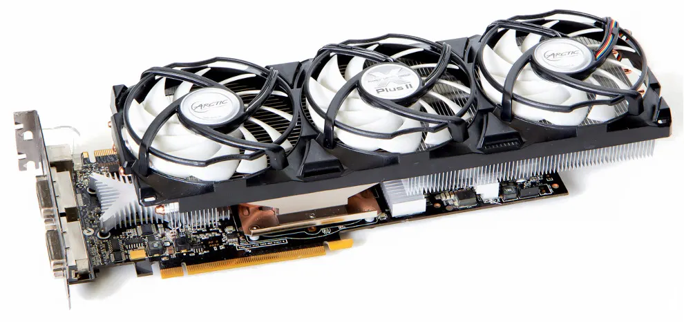
The use of heatsinks cooled by airflow reduces the temperature rise produced by a given amount of heat. Attention to patterns of airflow can prevent the development of hotspots. computer fans are widely used along with heatsink fans to reduce the temperature by actively exhausting hot air. There are also more exotic cooling techniques, such as liquid cooling. All modern-day processors are designed to cut out or reduce their voltage or clock speed if the internal temperature of the processor exceeds a specified limit.

Cooling may be designed to reduce the ambient temperature within the case of a computer, such as by exhausting hot air, or to cool a single component or small area (spot cooling). Components commonly individually cooled include the CPU, graphics processing units(GPU), and the northbridge.

In operation, the temperature of a computer's components will rise until the heat transferred to the surroundings is equal to the heat produced by the component, that is, when thermal equilibrium is reached. For reliable operation, the temperature must never exceed a specified maximum permissible value unique to each component. For semiconductors, instantaneous junction temperature, rather than a component case, heatsink, or ambient temperature is critical.

Mesh Generation:

Meshes are used for rendering to a computer screen and for physical simulation such as finite element analysis or computational fluid dynamics. Meshes are composed of simple cells like triangles because, e.g., we know how to perform operations such as finite element calculations (engineering) or ray tracing (computer graphics) on triangles, but we do not know how to perform these operations directly on complicated spaces and shapes such as a roadway bridge. We can simulate the strength of the bridge, or draw it on a computer screen, by performing calculations on each triangle and calculating the interactions between triangles.

Cut plane through the x-axis:

Cut plane through the y-axis:

Cut plane through the z-axis:

Mesh surface for the domain:

Numerical setting:

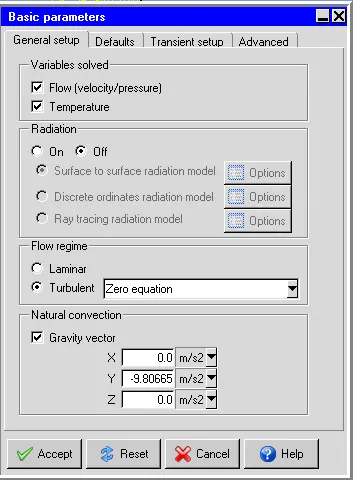
The general setup for basic parameters :

Basic parameters and choose the Zero equation turbulence model for the flow regime in the General setup tab.

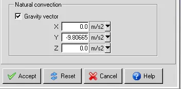
Set up the gravity vector :

Gravity acts in the negative x-direction in this problem. To set up the effects of gravity, toggle on the Gravity vector in the General setup tab. Enter the new values for the gravity vector as x = 0, y = -9.80665 and z =0.

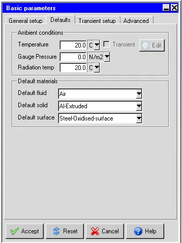
Defaults parameters :

Transient setup parameters

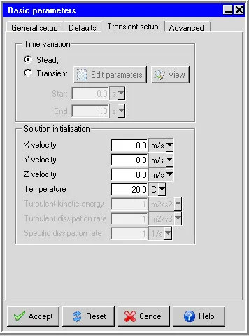
A steady-state simulation was considered in the simulation.

Advanced parameters in basic settings:

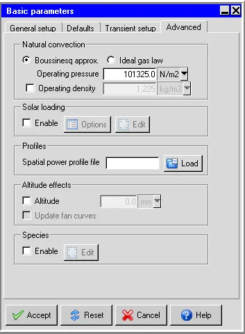
Set no of iterations and convergence criteria:

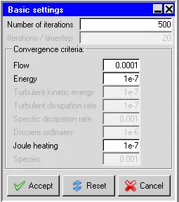
The total number of iteration was set to be 500 iterations and coming to the convergence criteria the flow was set to 0.0001 and joule heating, the energy was 1e-7, and the turbulent kinetic energy and turbulent dissipation rate were 1e-7

Parallel setting:

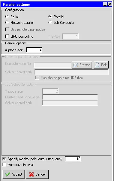
Advanced solver setup:

Select the Basic settings panel from the Solution settings branch of the tree and set the number of iterations to 300. Go to Advanced settings and specify Under-relaxation factors for Pressure, Momentum, and Temperature as 0.3, 0.7, and 1.0, respectively. Select Double for the Precision drop-down list. The recommended basic settings and advanced solver setup for this model are shown above.

Set up monitor points in the model:

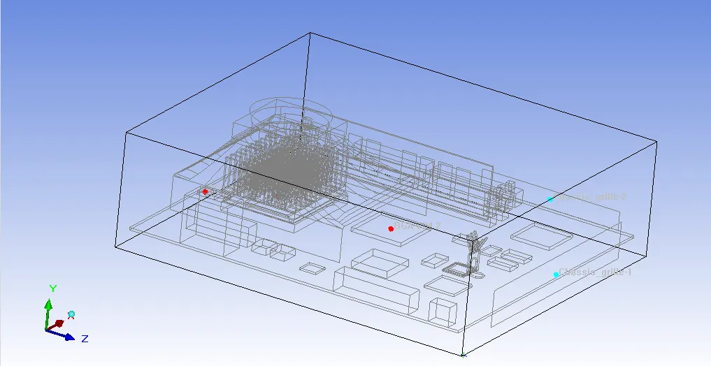
And monitor points were considered at the plates and blocks, chassis grill-1,2 and the red points represent the temperature monitor points and blue points represent the velocity monitor points in the domain

Solve the model:

There are no universal metrics for judging convergence, a good indicator is when the solution no longer changes with more iterations, and when the residuals have decreased to a certain degree. The default criterion is that each residual will be reduced to a value of less than 10^-3 except the energy residual, for which the default criterion is 10^-7. It is a good idea to judge convergence not only by examining residuals levels but also by monitoring relevant integrated quantities.

Residual plot:

Select the Basic settings panel from the Solution settings branch of the tree and set the number of iterations to 500. Go to Advanced settings and specify Under-relaxation factors for Pressure, Momentum, and Temperature as 0.3, 0.7, and 1.0, respectively. Select Double for the Precision drop-down list.

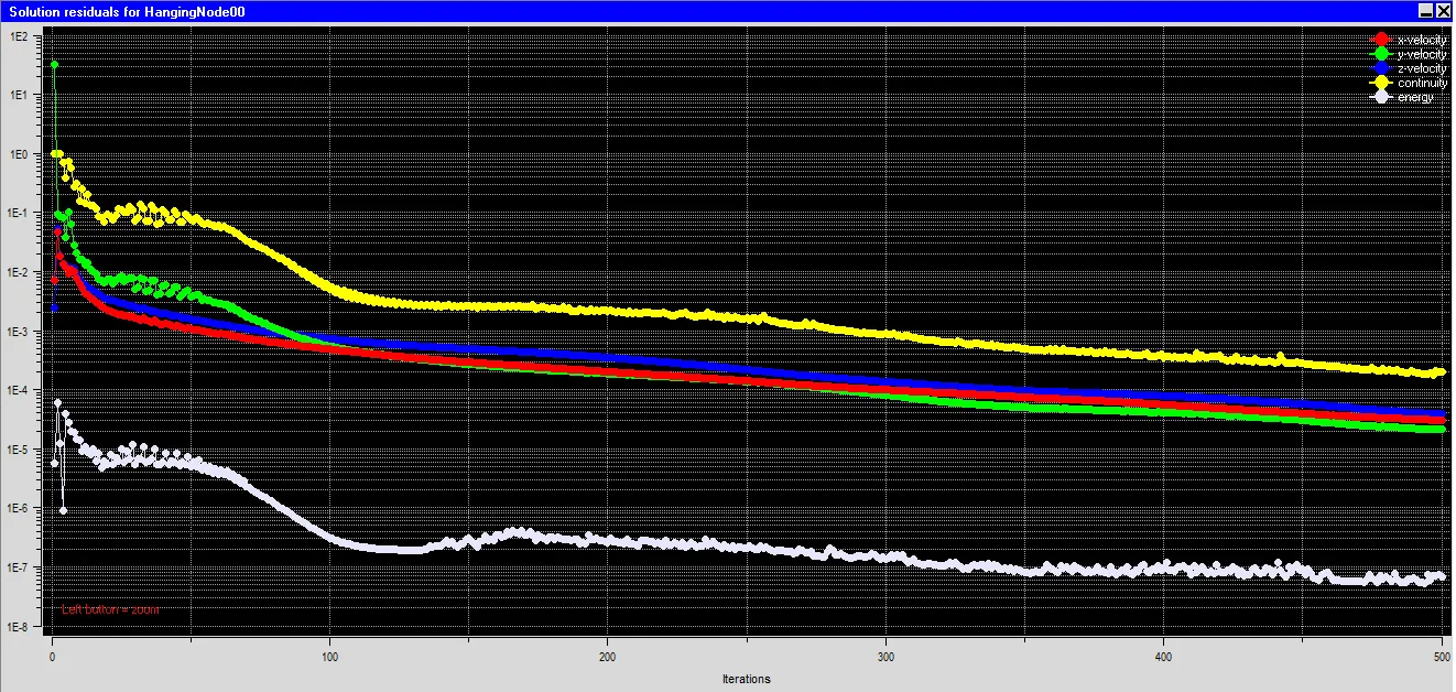
From the residual plot provided above it is clear that the simulation has reached the converged stage and also obtained the convergence, and they are no fluctuations in the plot.

Temperature monitoring points:

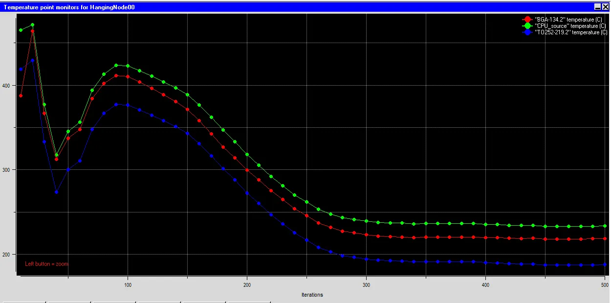
The temperature monitor points were considered on the CPU source, BGA, and TO252, the fluctuations can be seen in the starting of the simulation but after 300 iterations we can see the convergence has been obtained in the temperature plot.

• For the CPU source, we can see that the temperature on the object has been reached a final temperature of 240°C
• For the BGA, we can see that the temperature on the object has been reached a final temperature of 220°C
• For the TO252, we can see that the temperature on the object has been reached a final temperature of 196°C

Velocity monitoring points:

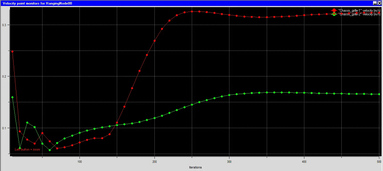
The temperature monitor points were considered on the chassis grill-1 and chassis grill-2 the fluctuations can be seen in the starting of the simulation but after 300 iterations we can see the convergence has been obtained in the velocity plot.

• For the chassis grill-1, we can see the final velocity on the object has been reached a final velocity of 0.35 m/sec
• For the chassis grill-2, we can see the final velocity on the object has been reached a final velocity of 0.17 m/sec

Plane cut:

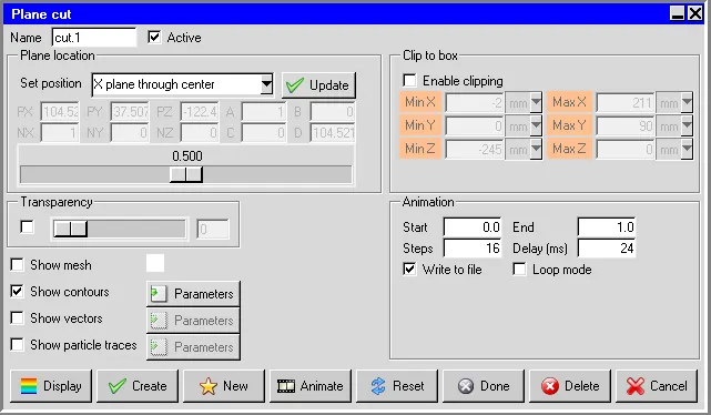
The cut plane was created for the hanging node model and the axis for the cut-plane used was the X plane through the center.

Pressure contour representation for the cut-plane:

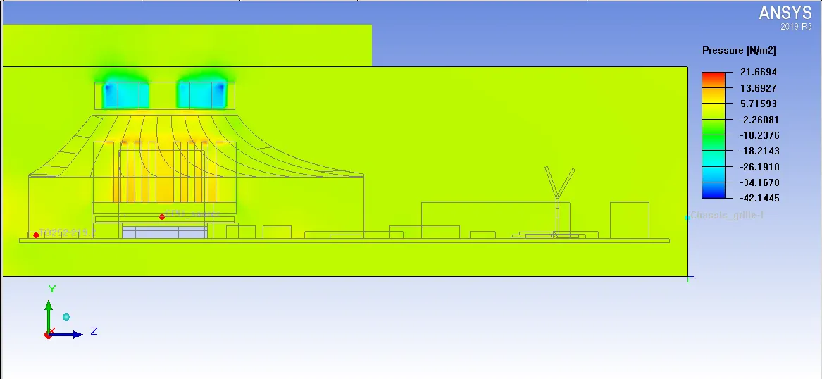
For the cut plane representation, we have shown the pressure contour on the X-plane for the model.

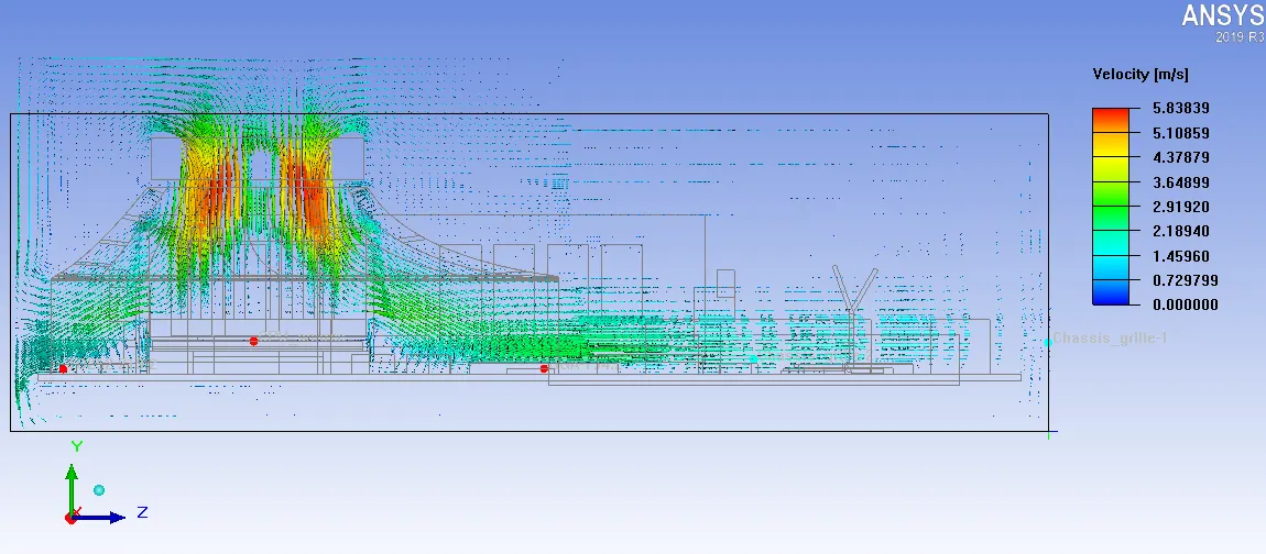
Vector plot:

The Vector plot was set to the x-plane through the plane and it is clearly seen that the inlet velocity for the opening was at the initial value of 0.72m/sec and a maximum velocity was at the value of 5.83m/sec was obtained in the domain and the velocity inside the domain was nearly at 2.91m/sec.

Temperature contour:

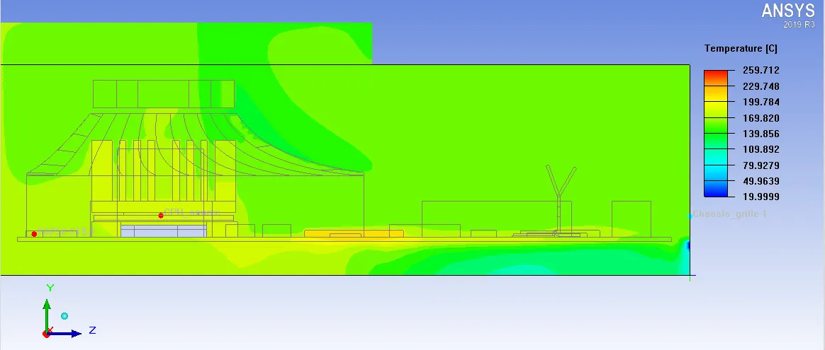
The Temperature Contour was set to position accordingly to the x plane through the plane and it is clearly seen that the initial temperature for the opening was at the 19.9°C and a maximum temperature of 259.7°C was obtained in the domain and the temperature inside the solid domain was nearly at 139.8°C.

Velocity contour:

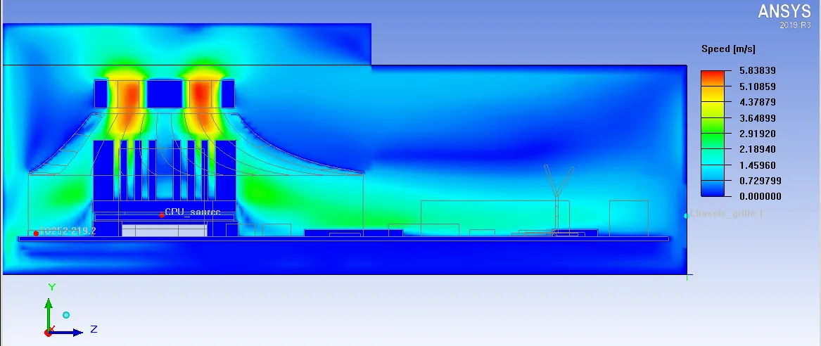
The Velocity Contour was set to position accordingly to the x-plane through the plane and it is clearly seen that the initial velocity for the opening was at the initial value of 0.72m/sec and a maximum velocity was at the value of 5.83 m/sec was obtained in the domain and the velocity inside the domain was nearly at 3.65 m/sec.

Pressure contour:

The Pressure Contour was set to position accordingly to the x-plane through the plane and it is clearly seen that the initial pressure for the opening was at the initial value of 2.26 N/m^2 and a maximum pressure was at the value of 21.6 N/m^2 was obtained in the domain and the pressure inside the domain was nearly at 5.71 N/m^2.

Negative pressure would mean that air is being sucked into your case from all the tiny gaps you can't control and don't have filters on, which means less efficient cooling over time. Aim for slightly positive-pressure, with slightly higher intake CFM than exhaust CFM.

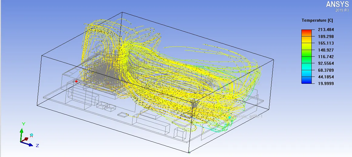
Stream particles profile:

A streamline is a path traced out by a massless particle as it moves with the flow. It is easiest to visualize a streamline. The stream-lines profile was shown below on the total domain in the hanging node.

Object face:

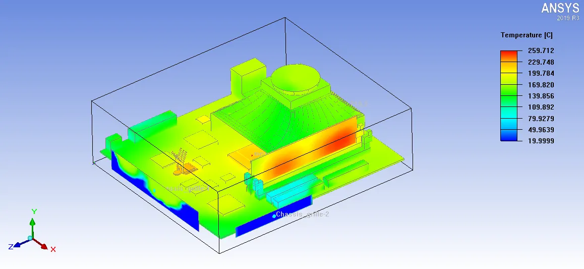
The overall temperature distribution throughout the hanging node model was shown in the above Figure.

Object face to display velocity contour on overall Hanging Node Model:

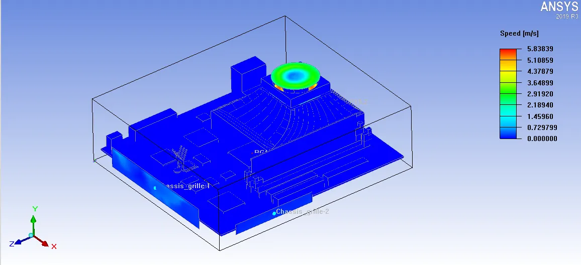
The overall velocity distribution throughout the hanging node model was shown in the above Figure.

Object face to display Pressure contour on overall Hanging Node Model:

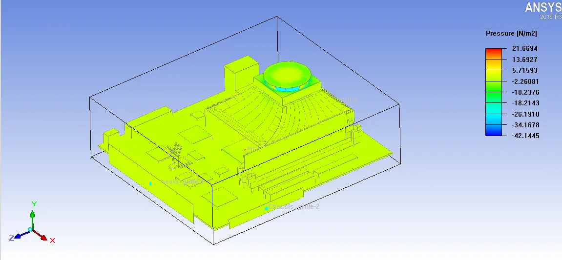
The overall Pressure distribution throughout the hanging node model was shown in the above Figure.

Conclusion:

• We have successfully performed the simulation analysis for a hanging node model and obtained the results by post-processing. And separately meshed assemblies have been employed to reduce the overall mesh count in the domain.
• Parameters like temperature, pressure, and velocity were plotted. And monitor points were considered at the plates and blocks, chassis grill-1,2 to obtain the temperature and velocity that has generated in the model.