Week 6.1 - Setting up a model (Electronic enclosure)

Aim:

To simplify the given CAD model of an electronic enclosure assembly and perform thermal analysis of the same.

Objective:

• The given CAD model is simplified into an Icepak model using the commands available in ANSYS SpaceClaim.
• The model is imported into ANSYS Icepak using a suitable workflow created in ANSYS Workbench.
• Appropriate heat generation values are assigned to various objects in the model.
• The model is meshed using the non-conformal meshing technique.
• The three-dimensional steady-state governing equations for the model are solved on the computational mesh, for flow and temperature.

Introduction:

The heat sink is one of the most popular devices used in the electronic industry for managing the thermal dissipation of electronic devices. Unlike a fan which requires an electric current to function, a heat sink is a passive device and doesn't require any external energy. It is placed in direct contact with the electronic device whose temperature is to be regulated. It conducts the heat generated by the device and transfers it to the coolant fluid or air by convection. In the current project, natural convection drives the ambient air through the enclosure assembly. At a steady state, the total heat generated by the model is carried away by the air current created due to natural convection. This kind of simulation is often performed in the electronic industry to determine if a particular design is able to manage the thermal dissipation in its electronic circuit effectively.

Geometry simplification:

1.The images attached below show the given CAD model of the electronic enclosure assembly.

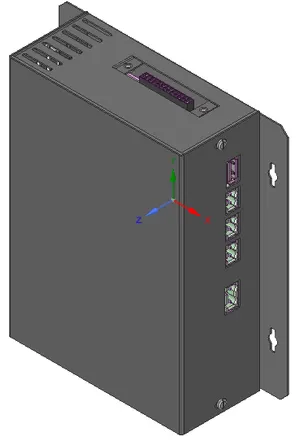
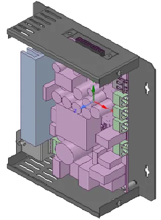
The following steps are used to convert the given CAD model into an Icepak model:

Since the extensions on the outer cover don't affect the flow or thermal analysis in any manner, they can be removed from the geometry using the "Split Body" command available in SpaceClaim.

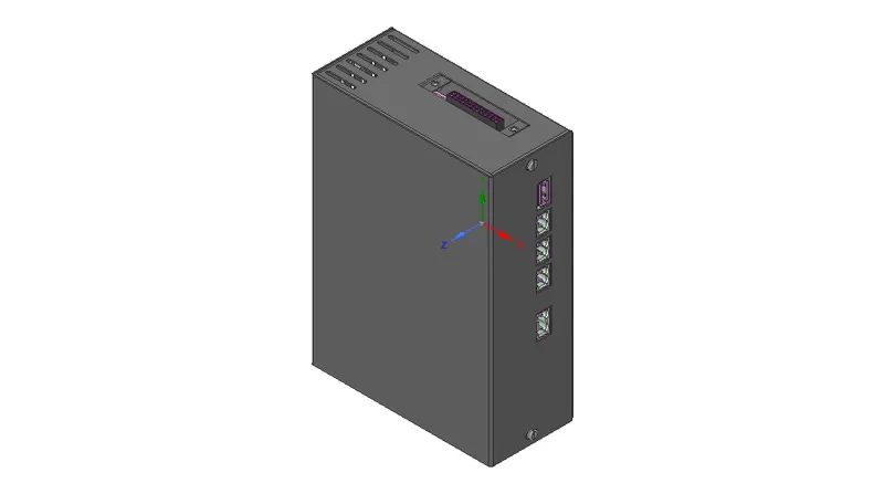
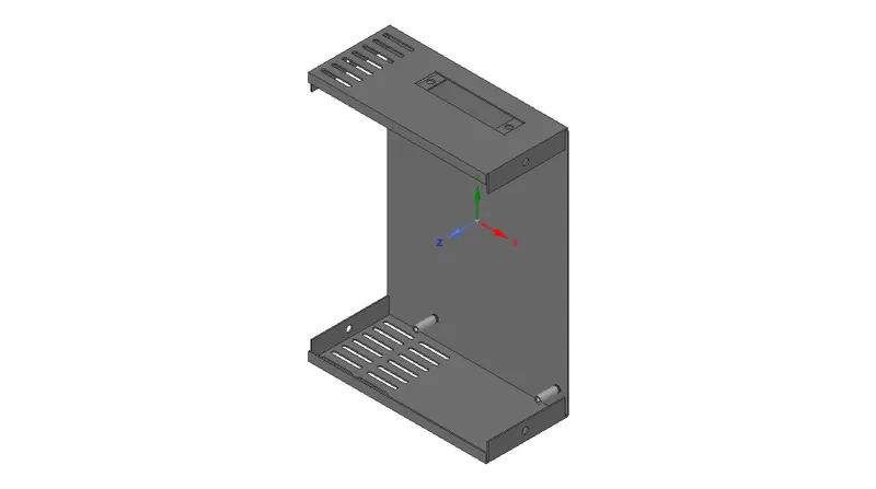
2. The bottom cover of the enclosure is opened in a separate design window. The image attached below shows the CAD geometry of the same.

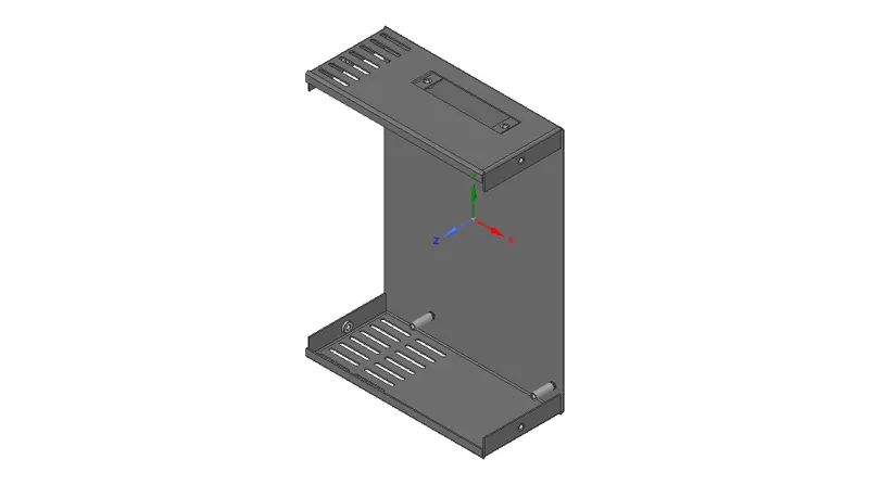
The following steps are used to convert the CAD geometry (shown above) into an Icepak geometry:

2.1. All the round edges and washers are removed from the geometry.

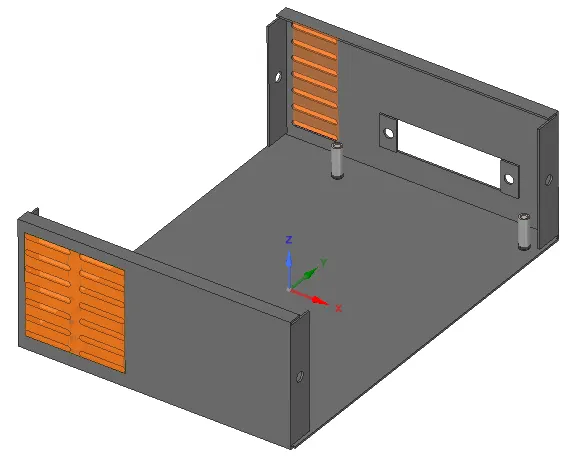
2.2. Using the "Opening" and "Grille" commands, two Icepak-grilles are defined in the geometry as shown in the image attached below.

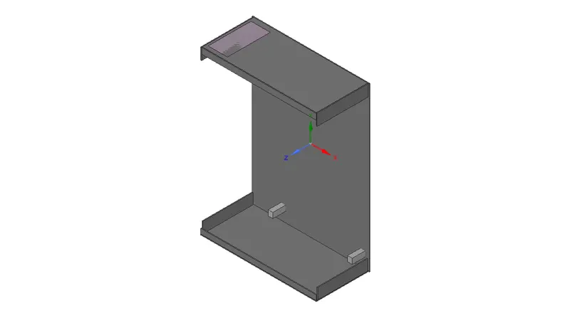
2.3. The bottom cover is split using the "Split Body" command and each of the resultant parts is then simplified into an Icepak object using the "Icepak Simplify" command with level 0 (bounding box) simplification type. The image attached below shows the bottom cover after simplification.

3. The part corresponding to PCB and electronic components is opened in a separate design window (shown in the image attached below) for simplification.

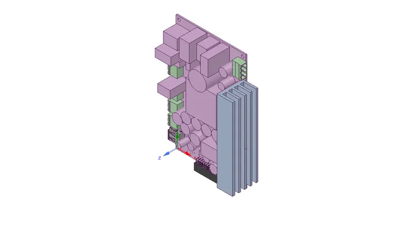
The following steps are used to convert the CAD geometry (shown above) into an Icepak geometry:

3.1. The part is divided into multiple parts by using the "Split Body" command with the top and bottom planes of the PCB. This separates most of the components from each other.

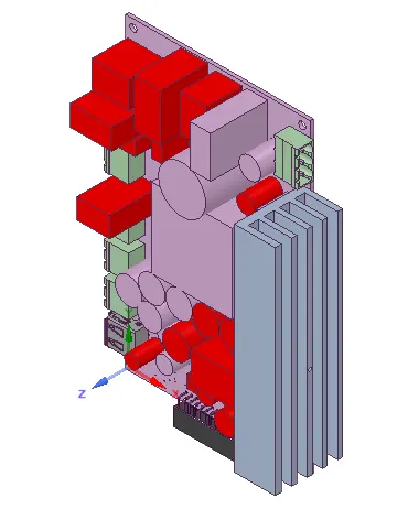
3.2. The "Identify Objects" command is used to allow ANSYS SpaceClaim to identify and convert different objects in the model into Icepak objects. The image attached below shows the different objects (highlighted in red color) that have been identified by ANSYS SpaceClaim for conversion to Icepak objects.

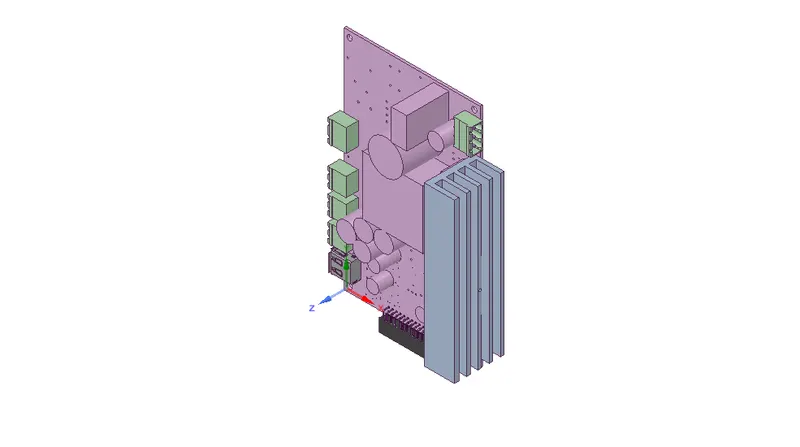
3.3. The remaining non-Icepak objects are shown in the image attached below.

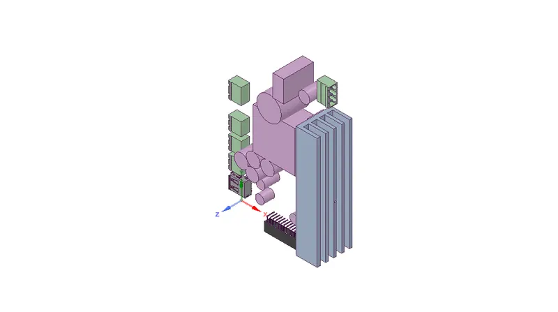
3.4. The PCB is simplified using the "Icepak Simplify" command with level 0 (bounding box) simplification type. The remaining non-Icepak objects are shown in the image attached below.

3.5. The remaining non-Icepak objects are simplified using the "Icepak Simplify" command with different simplification types. Some of the objects are first separated into multiple objects using the "Split Body" command and selecting appropriate planes. The images attached below show some of the objects before and after simplification.

(a) CAD geometry (before simplification)

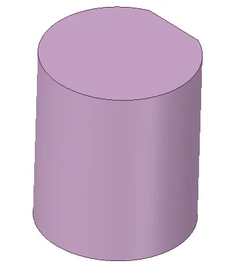
(b) Icepak geometry (after level 1 (cuboid, cylinder fit) simplification)

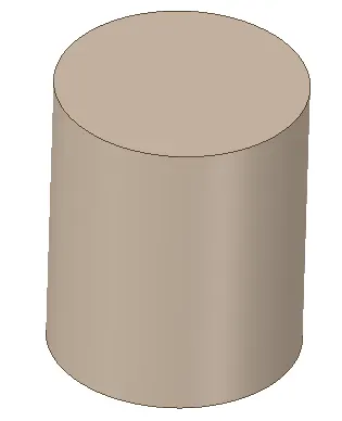
(a) CAD geometry (before simplification)

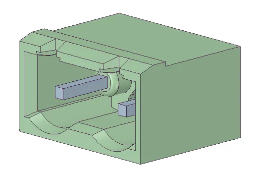
(b) Icepak geometry (after level 0 (bounding box) simplification)

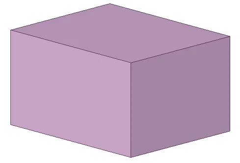
(a) CAD geometry (before simplification)

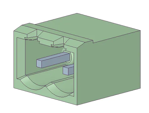
(b) Icepak geometry (after level 0 (bounding box) simplification)

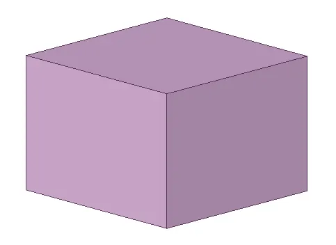
(a) CAD geometry (before simplification)

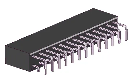
(b) Icepak geometry (after level 0 (bounding box) simplification)

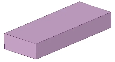
(a) CAD geometry (before simplification)

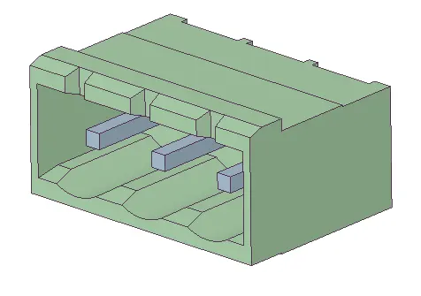
(b) Icepak geometry (after level 0 (bounding box) simplification)

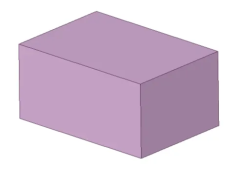
(a) CAD geometry (before simplification)

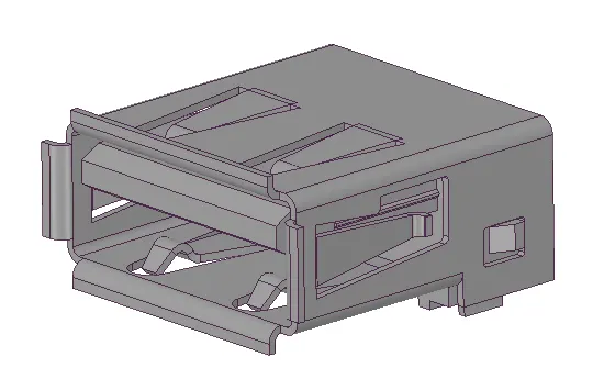
(b) Icepak geometry (after level 0 (bounding box) simplification)

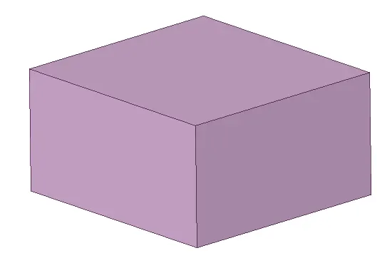
(a) CAD geometry (before simplification)

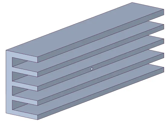
(b) Icepak geometry (after level 1 (cuboid, cylinder fit) simplification)

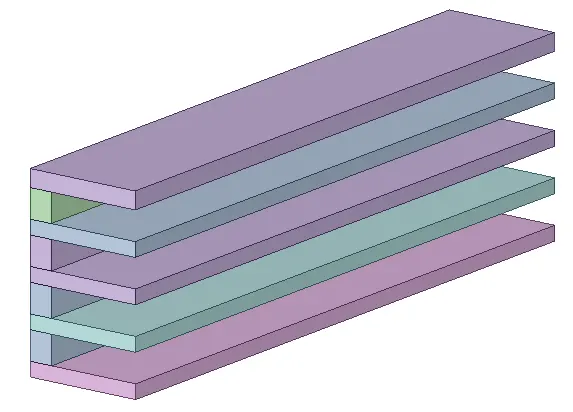
The image attached below shows the part corresponding to PCB and electronic components after simplification.

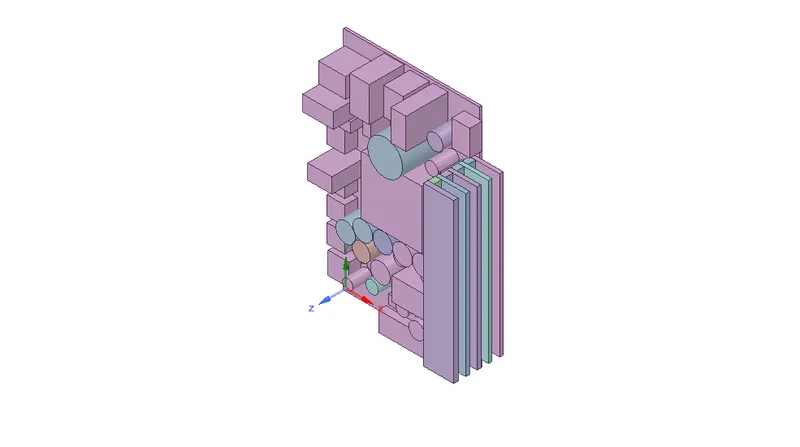
4. The remaining non-Icepak objects in the model are shown in the image attached below.

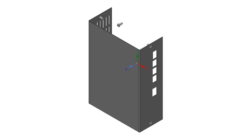
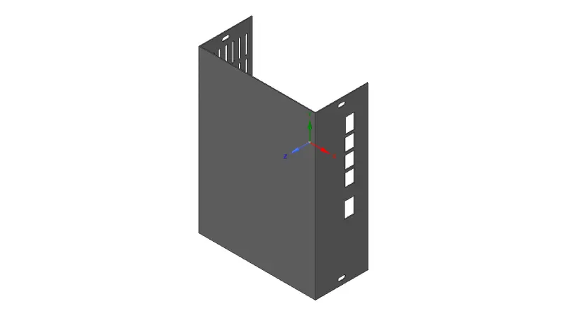
5. All the round edges, washers and screws are removed from the geometry as shown in the image attached below.

6. The part corresponding to the top cover is opened in a separate design window as shown in the image attached below.

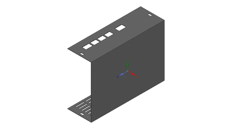
The following steps are used to convert the CAD geometry (shown above) into an Icepak geometry:

6.1. Using the "Opening" and "Grille" commands, an Icepak-grille is defined in the geometry as shown in the image attached below.

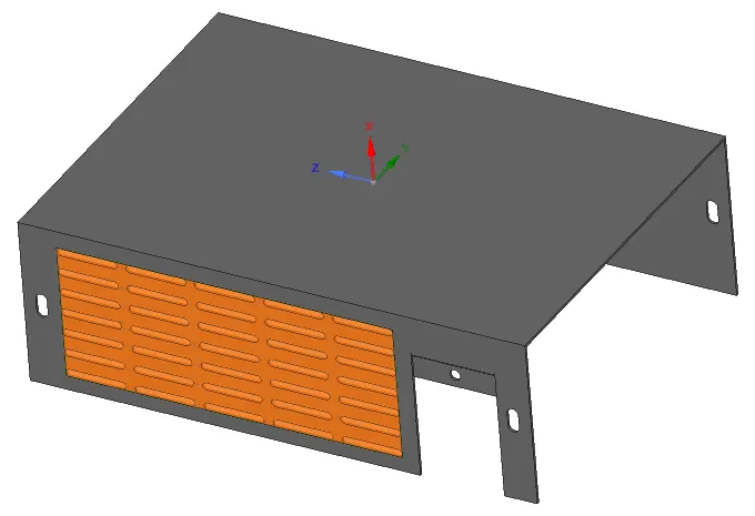
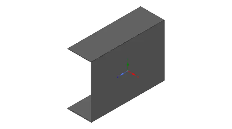
6.1. The object is split into multiple (three) objects using the "Split Body" command and selecting a plane parallel to the YZ plane, in order to make the simplification more convenient. Each of the resultant objects is then simplified into an Icepak object using the "Icepak Simplify" command with level 0 (bounding box) simplification type. The image attached below shows the top cover after simplification.

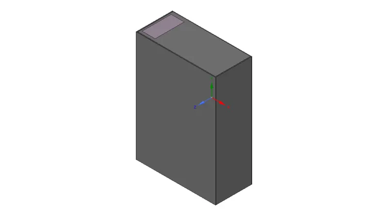
The image attached below shows the complete simplified geometry of the electronic enclosure assembly which can be imported to ANSYS Icepak.

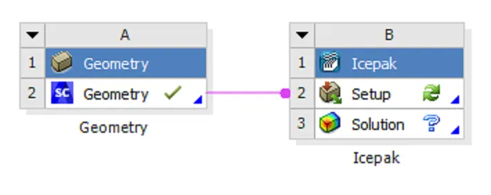
In order to import the simplified geometry of the enclosure assembly (shown above) into ANSYS Icepak, a workflow with the following two standalone systems is created in ANSYS Workbench:

A. Geometry

B. Icepak

The two standalone systems are linked such that the geometry created/imported/simplified in the "Geometry" tab of the system "A" ("Geometry") is transferred to the "Setup" tab of the system "B" ("Icepak"). The image attached below shows the workflow created in ANSYS Workbench.

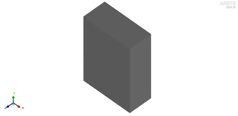
Upon opening the "Setup" tab of the system "B" ("Icepak"), the simplified geometry is imported into ANSYS Icepak as shown in the images attached below.

The following steps are utilized to ensure that the entire computational domain is meshed properly:

1. The small objects in the model that are located on the surface of the PCB but don't affect the flow/thermal field within the computational domain are deactivated for analysis.

2. The objects in the model that have their geometries interfering with each other are identified and moved apart.

The images attached below show the complete geometry of the model, which is now ready for the meshing procedure.

Meshing:

The computational domain is discretized using Hexa unstructured mesh with the following settings:

1. Max element size

1.1. X: 6.08005 mm

1.2. Y: 8.46005 mm

1.3. Z: 2.79005 mm

2. Mesh parameters: Normal

3. Min elements in gap: 3

4. Min elements on edge: 2

5. Max size ratio: 2

6. Mesh assemblies separately: Enabled

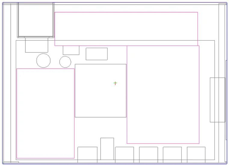
In order to reduce the overall mesh count by preventing mesh bleeding, the non-conformal meshing technique is applied. Assemblies are defined around key objects (that affect the flow/thermal field within the computational domain) in the model. The image attached below shows the different assemblies defined in the model.

The generated mesh yields 530551 elements and 562452 nodes. The images attached below show the computational mesh plotted on three mutually perpendicular planes, each passing through the center of the cabinet.

1. X plane through center

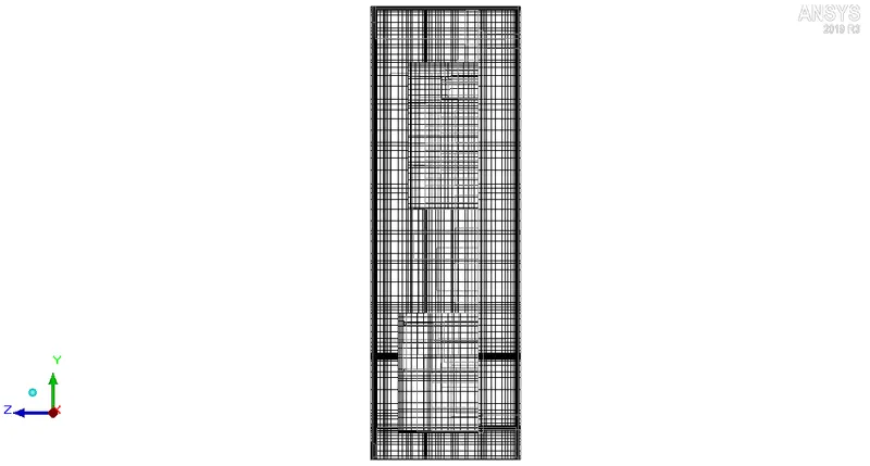
2. Y plane through center

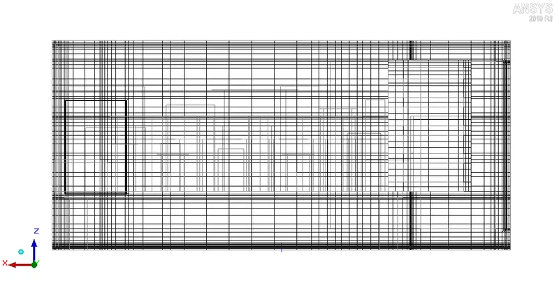
3. Z plane through center

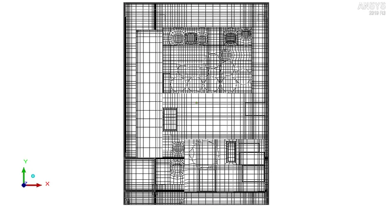
Visually the mesh appears to be fine. The images attached below show the histograms with number of elements plotted along the X-axis and quality measures plotted along the Y-axis.

1. Face alignment

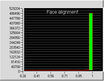
Values less than 0.05 indicate the presence of severely distorted elements in the mesh. For the current mesh, the minimum value of face alignment is 0.262783 which indicates that the mesh elements aren't severely distorted.

2. Volume

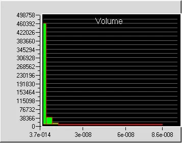
For a double precision solver, the minimum cell volume shouldn't be less than 1e-15 m3 otherwise the solver may face issues. The minimum cell volume in the current mesh is 3.71579e-14 m3 and hence the mesh elements aren't small enough to cause problems in the solver.

3. Skewness

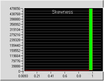
A skewness of 0 indicates that the mesh element is degenerate whereas a skewness of 1 indicates that the mesh element is ideal (equiangular/equilateral). For the current mesh, the minimum value of skewness is 0.00930464 which indicates that no element in the mesh is degenerate.

V. Solver

The three dimensional steady-state Navier-Stokes equations for the model are solved within the computational domain for flow and temperature fields, using the Fluent solver available in ANSYS Icepak. The following settings are applied to the solver:

1. Variables solved: Flow (velocity, pressure) and Temperature

2. Radiation: Off

3. Flow regime: Turbulent (Zero equation)

4. Time variation: Steady

5. Solution initialization

5.1. X velocity: 0

5.2. Y velocity: 0.000980665 m/s

5.3. Z velocity: 0

5.4. Temperature: ambient (20 deg. C)

6. Number of iterations: 2000

7. Convergence criteria

7.1. Flow: 1e-7

7.2. Energy: 1e-7

7.3. Joule heating: 1e-7

8. Configuration: Parallel

9. Number of processors: 4

10. GPU computing: Enabled

11. Number of GPUs: 1

12. Precision: Double

The image attached below shows (in red color) the objects in the model that have been assigned a power generation of 10 W, each.

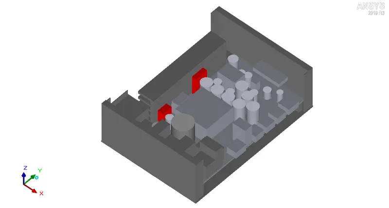
Hence the total power generated by the model is 20 W.

VI. Results

In the current section, simulation results are discussed.

1. Residuals

The residuals for the following equations are plotted against the number of iterations:

i. Continuity equation

ii. X-Momentum equation

iii. Y-Momentum equation

iv. Z-Momentum equation

v. Energy

The image attached below shows the residuals plotted against the number of iterations.

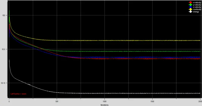
The plot shows that the residuals don't change appreciably after 750 iterations thereby indicating that the solution has reached a steady state. For the current project, the simulation is run for 2000 iterations even though the solution has already reached steady state after 750 iterations. Henceforth the simulation results after 2000 iterations are considered as steady-state results.

2. Temperature-monitor plot

Two temperature monitors are defined to measure the average surface temperatures of the two heat sources in the model. The image attached below shows the outputs from the two temperature monitors as a function of the number of iterations.

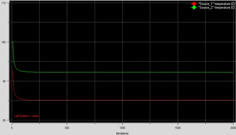
The image shows that beyond 250 iterations there is no appreciable change in the average surface temperatures of the two heat sources in the model. Hence according to the temperature-monitor plot also the simulation results after 2000 iterations can be considered as steady-state results. The following steady-state temperatures are attained by the two heat sources in the model:

i. PWR_V2_23062016_RIGHT_SW0005791 (Source_1): 85.06 deg. C

ii. PWR_V2_23062016_RIGHT_SW000572 (Source_2): 92.24 deg. C

3. Velocity contours

The image attached below shows the steady-state velocity contours plotted on the Z-plane through center.

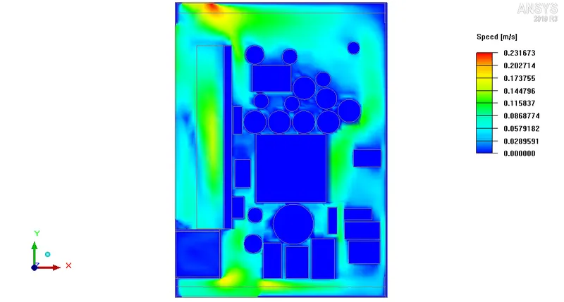
The contour plot shows that the air inside the enclosure assembly is in motion and the electronic components on the PCB (capacitors, heat-sink etc.) affect its flow. According to the contour-legend the maximum air-velocity within the computational domain on the Z-plane through center is 0.232 m/s.

4. Velocity vectors

The image attached below shows the steady-state velocity vectors plotted on the Z-plane through center.

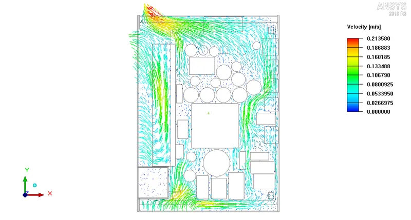
The vector plot clearly shows the direction of motion of air within the computational domain, as it (air) enters into the enclosure assembly through the bottom grille, moves over the electronic components on the PCB and finally leaves through the top grille. This upward motion of air against gravity (which is directed along the negative Y-axis) can be attributed to natural convection. The velocity vectors also clearly show the recirculation of air through the side grille.

5. Temperature contours

The image attached below shows the steady-state temperature contours plotted on the Z-plane through center.

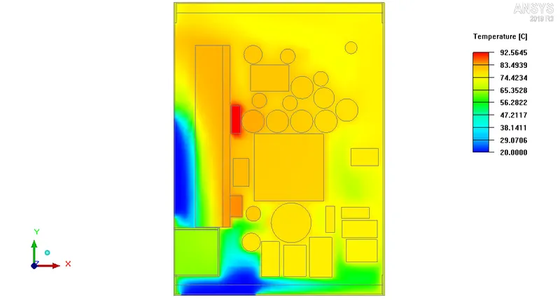
The contours show that the air inside the enclosure assembly is at a higher temperature due to convection heat transfer between the electronic components and the air. The hot air rises up against gravity (directed along the negative Y-axis) and finally leaves the enclosure assembly through the top grille and the upper part of the side grille. This drives cool air (at ambient temperature) inside the enclosure assembly through the bottom grille and the lower part of the side grille. The cool air picks-up the heat generated by the model, rises up and leaves through the top grille and the upper part of the side grille. In this manner natural convection drives air through the enclosure assembly and allows for effective thermal management of the saem (enclosure assembly).

6. Object face temperature contours

The image attached below shows the steady-state object face temperature contours plotted on all the objects in the model that are located within the housing except the PCB supports.

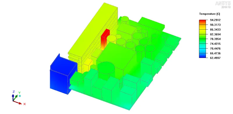
The contours show that the highest steady-state temperature is attained by one of the two heat sources in the model. Due to the thermal dissipation of heat sources, the objects that are located closer to them are hotter as compared to the objects that are located far away.

7. Particle traces

The image attached below shows the steady-state particle traces for 60 particles distributed uniformly within the computational domain.

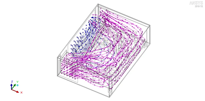
The image shows the pathlines traced by the air particles originating at the bottom grille (shown in pink color) and the side grille (shown in blue color), at a steady state. The pink-colored particle traces show that the air particles entering into the enclosure assembly through the bottom grille flow over the electronic components on the PCB and finally leave through the top grille. Similarly, the blue-colored particle traces show that the air particles entering into the enclosure assembly through the side grille flow over the heat sink and leave through the upper part of the side grille. The animation attached below shows the steady-state particle traces (colored by temperature) for 60 particles distributed uniformly within the computational domain. The color of the particle trace at a particular location indicates the temperature of the air particle at that location.

Conclusion:

In the current project, the given CAD model of an electronic enclosure assembly was simplified into an Icepak model using the commands available in ANSYS SpaceClaim. The model was imported into ANSYS Icepak by creating a suitable workflow in ANSYS Workbench. The model was meshed using a non-conformal meshing technique and steady-state simulation was performed with appropriate solver settings. The following conclusions can be drawn from the simulation results:

1. Both the residual plot and the temperature monitor plot indicated that the simulation results after 2000 iterations can be considered as steady-state results.

2. One of the two heat sources in the model attains the maximum steady-state temperature (92.24 deg. C) out of all the assembly components.