Week 5 - Turbulence modelling challenge

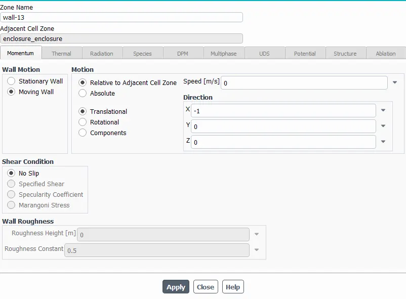
Aim: To performs a 3D simulation and explain the recirculation region using velocity vectors to the given model by Consider the flow direction of air, the ball is traveling opposite to it at 60m/s.

Introduction:

Reynolds Number:

The ratio of inertia force to viscous force is called as Reynolds number.

`Re = frac(rho*V*D)(mu)`

Types of Flows:

1. Laminar Flow:

• Occur at low Reynolds number
• Viscous forces are dominant
• Characterized by smooth, constant fluid motion.

2. Turbulent Flow:

• Occurs at high Reynolds number
• Inertia forces are dominant.
• Produce chaotic eddies, vortices and other instabilities.

3. Transition Flow:

• Energy and momentum transfer are strongly influenced by either inertial or non-linear effects that are unique to the simulation.

Various turbulence models:

• Spalart-Allmaras Model:
  
  The Spalart–Allmaras model is a one-equation model that solves a modeled transport equation for the kinematic eddy turbulent viscosity. The Spalart–Allmaras model was designed specifically for aerospace applications involving wall-bounded flows and has been shown to give good results for boundary layers subjected to adverse pressure gradients. It is also gaining popularity in turbo machinery applications.
  
  
• K-Epsilon Model:
  
  K-epsilon turbulence model is the most common model used in computational fluid dynamics (CFD) to simulate mean flow characteristics for turbulent flow conditions. It is a two-equation model which gives a general description of turbulence by means of two transport equations (PDE's). The original impetus for the K-epsilon model was to improve the mixing-length model, as well as to find an alternative to algebraically prescribing turbulent length scales in moderate to high complexity flows.
  1. Standard k-epsilon Model: Basic form suitable for many applications.
  2. Realizable k-epsilon Model: Includes additional equations to improve predictions, especially for complex flows.
  3. RNG k-epsilon Model: (Re-Normalization Group): Another variant that aims to improve predictions.
  
  
• K- Omega Model:
  
  In computational fluid dynamics, the k–omega turbulence models a common two-equation turbulence model that is used as a closure for the Reynolds-averaged Navier–Stokes equations (RANS equations). The model attempts to predict turbulence by two partial differential equations for two variables, k, and. The first variable being the turbulence kinetic energy (k) while the second () is the specific rate of dissipation (of the turbulence kinetic energy k into internal thermal energy).
  1. Standard k-omega Model: Basic form
  2. SST (Shear-Stress Transport) k-omega Model: Blends features of both k-epsilon and k-omega models, providing accurate predictions for a wide range of flows.

Direct Numerical Simulation (DNS) is a computational approach in fluid dynamics where all scales of motion, including the smallest turbulent scales, are resolved numerically. Kolmogorov's scale is a concept in turbulence theory that describes the smallest scale of turbulence where dissipation occurs. In the context of DNS, there are challenges and limitations associated with resolving the Kolmogorov scale, making DNS impractical for certain types of flows. Here are some reasons why DNS may not be feasible according to Kolmogorov's scale.

• computational cost: The Kolmogorov scale is minimal, especially in high Reynolds number flows where turbulence is prevalent. To resolve the Kolmogorov scale, very fine computational grids are required. This leads to an enormous number of grid points, making DNS computationally expensive and often beyond the current capabilities of available computing resources.
• Time step: To accurately capture the evolution of turbulent structures, DNS simulations must use very small-time steps. This increases the total number of time steps needed for a simulation and further contributes to the computational cost.
• Reynolds number consideration: Turbulent flows are characterized by their Reynolds numbers, which are a measure of the ratio of inertial forces to viscous forces. In high Reynolds number flows, the Kolmogorov scale becomes minimal. Resolving such small scales computationally is challenging and, in many cases, impractical.
• Storage and memory requirement: DNS requires storing the velocity field at each grid point and at each time step. The vast amount of data generated in DNS simulations, especially when resolving small scales, requires significant storage and memory resources.

Procedure:

Geometry:

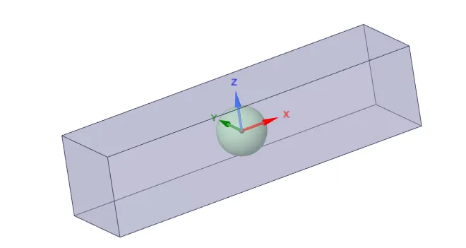
The given geometry is loaded into the Ansys spaceclaim, without making any changes to the model.

Mesh:

Here, the model is meshed meshed with an element size of 1 mm.

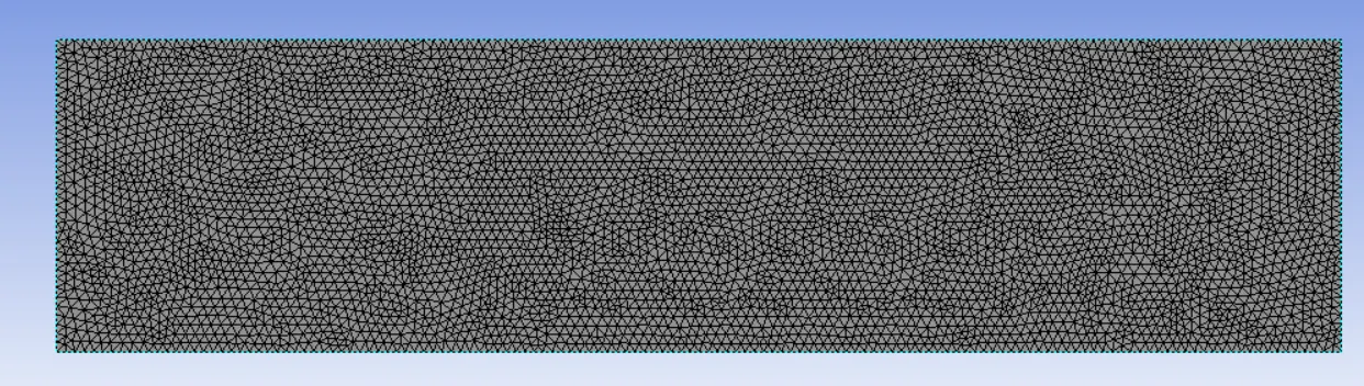
And the faces are named as inlet, outlet, Fairfield, symmetry-wall, golf_ball

Setup:

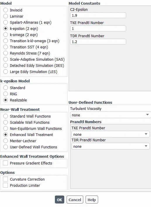
Viscous Model:

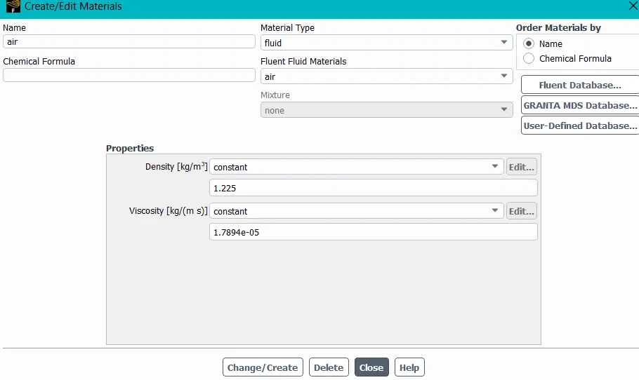
Material:

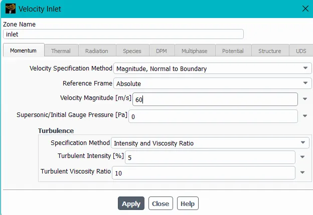
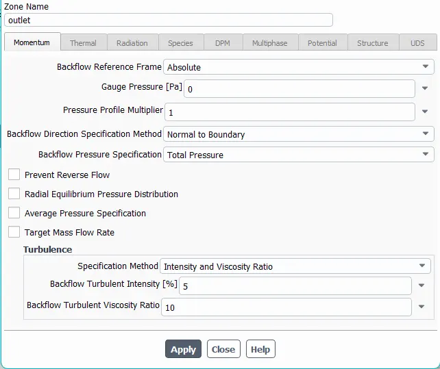
Boundary conditions:

• inlet
  
• outlet:
  
• golf_ball
  
• And the symmetry_walls are treated as symmetry type.

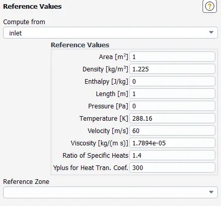
Reference values:

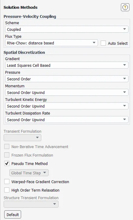
Methods:

Results:

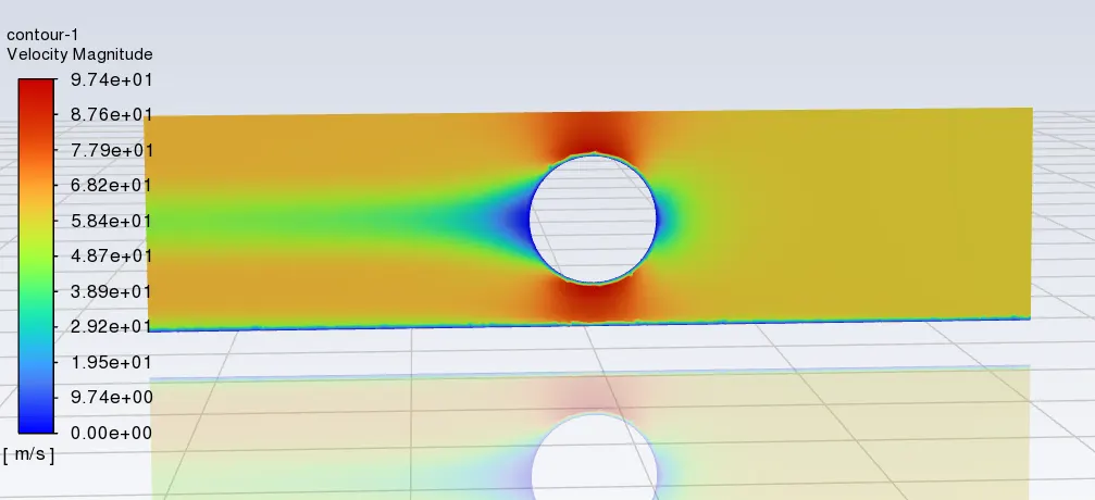
Velocity contour:

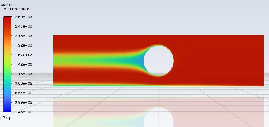
Pressure contour:

velocity vector:

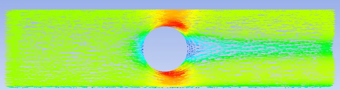
Here, the velocity vectors will determine the direction of the ball, that the vectors flow going downwards at the wake region.

The ball separates the vector flow that causes high drag coefficient, then the vectors collides with the downward vector flow causing low drag coefficient at the wake region.