Week 5 - Turbulence modelling challenge

Turbulence Model:

Reynolds No.: It is the ratio of the inertial force to the viscous flow of the fluid

`Re=(rho*V*l)/mu`

The fluid flow is classified into different categories based on the Reynolds no.

• Laminar flow: In this type, fluid flows in streamline fashion. In laminar flow the velocity of fluid remains same with less deviation across streamlines.
• Turbulent Flow: this type of flow is most commonly observed in at the trailing edge of the aeroplane wing tip. Turbulent flow is chaotic in nature, by studying and simulating the flow we could develop various model which is of great use. Further, turbulent flow domain is not yet fully being explored and research is still going on.
• Transition flow: This type of flow is observed when a laminar flow is converted into turbulent flow at the trailing edge of any body. Energy & momentum transfer are strongly influenced by either inertial or non-linear effects that are unique to the simulation.

Importance of turbulence:

• In a Turbulent flow there are two main phenomenon which is of great interest i.e. Energy dissipation & noise generation.
• Turbulent flow is highly acoustic in nature. So determining the flow characteristic of turbulent flow is very difficult.
• After long research scientist came up with coherent structures which are associated with the turbulent flow. These structure helped the scientist to model the turbulent flow i.e. Vortices.

Eddy formation in turbulent flow:

• Consider the flow over the flat plate, we find that at the leading edge the flow is attached to the platre but after attaining critical Reynolds number the flow starts to transition into turbulent flow.
• Turbulent flow is observed by visualizeing large eddy formation by gaining momentum energy of flow. This large eddy after gaining enough momentum becomes unstable and gives rise to smaller eddies.

• The smaller eddies come together to form large eddies sometimes, but mostly they dissiociates by giving heat energy. This phenomenon is known as energy cascading.

Types of eddies:

A) Large eddies:

• Size of large eddies is directly proportional to the ratio of the characteristics length to the free stream velocity.

size of large eddies `prop L/U`

• Energy source for the large eddies is from the momentum gained from mean flow velocity.

B) Smaller eddies

• Size of smaller eddies is directly proportional to the ratio of the characteristics length to the three fourth power of the Reynolds number.

Size of small eddies `prop L/(Re)^(3/4)`

• Energy for the smaller eddies is obtained from the larger eddies.

Identify the scale of smaller eddies:

Inorder to identify the scale of the eddies Kolmogrov developed two types of scale to measure the eddies they are

(i) Kolmogrov length scale: It is the scale which is used to identify the size of the eddy

`eta=(nu^3/(epsi))^(1/4)` where, `epsi`= dissipation of turbulent kinetic energy

`epsi=U^3/L`

(ii) Kolmovgrov time scale: which is used to identify the turn around time of the eddies.

`tn=(nu/epsilon)^(1/2)`

Ratio of the largest eddies to the smallest:

`L/eta = L/((nu^3/epsi)^(1/4) )=(L/nu^(3/4))*(U^(3/4)/L^(1/4))=((L*U)/nu)^(3/4)=Re^(3/4)`

• As the Reynolds no. increases the difference between the largest and the smallest eddies also increases.

Modelling turbulent flow:

• If the vortex generated is large then they can be resolved using large sized mesh grid, but if the vortex generated is small then we need to refine the mesh.
• Which increases the no. of mesh count and in turn it becomes computationally expensive.
• So the major challenge is to resolve the small scale structures.

In order to resolve such small scale structures we have three types of methods

• DNS (Direct Numerical Simulations)
• LES (Large Eddy Simulation)
• RANS (Reynolds Averaged Navier Stokes)

(i) DNS:

• It solves the Navier stokes equations at a very small scale.
• According to kolmogrov scale, inorder to resolve the smallest eddies we require the mesh size to be smaller then this.

`eta=(1/(Re)^(3/4))`

• If we consider 3D simulation then the gride size should be smaller then this

``eta=(1/(Re)^(9/4))``

no. of elements `propRe^(9/4)`

• This leads to large no. of elements in 3D simulations, so is usually not used in industrial applications
• But for 2D simulation in research purpose, it is still preferred.

(ii) LES:

• From the name it is clear that it is mainly used in large eddy simulation only.
• Smaller eddies is also modelled using sub grid method
• In this methods the number of elements is not as large as it is mainly dependent on the characteristics length and velocity alone. But since the smaller eddies are mostly neglected the results obtained are less accurate.
• It is usually used in simulation problems for combustion and acoustics.

(iii) RANS:

• DNS being computationally expensive & LES being less accurate by neglecting small eddies, thius give rise to new method called RANS.
• This method is widely used in most of the commercial software packages like Ansys, Star CCM+ etc.
• RANS uses Reynolds decomposition method to resolve the problems.

Reynolds Decomposition:

• It states that the fluctuating component can be resolved into average component and fluctuating component.

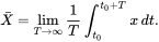
The mean (time-averaged) component () and the fluctuating component ()

• When we consider time averaging, as the time tends to infinity the fluctuating terms die out i.e. zero.
• Applying Reynolds decomposition to Navier Stokes equation for incompressible flow
• Time averaging of the average quantity is the same, and that of the fluctuating terms is zero as time tends to infinity. Hence continuity equation is averaged
• Similarly the same method can be applied to momentum and energy equation as well.
• For compressible flow at low Reynolds number the density fluctuation term becomes negligible, but for hypersonic flows the density fluctuation becomes very high.
• Hence the Reynolds time averaging method is not used instead mass averaging or Favre averaging method is used.
• By using Reynolds averaging we obtain one additional term known as Reynolds stress term. Without considering the Reynolds stress term the equation is not closed.
• Additional equations are required to solve the Reynolds stress terms.

Models available to solve the Reynolds stress terms:

(i) First order model:

• It uses first order PDE’s to solve the Reynolds stress term. For industrial application the first order model of two equation type is most commonly used.
• It assumes average turbulent flow field to be similar to corresponding laminar flow.
• Zero equation model:
  • No PDE is used to solve for turbulent viscosity, hence it fails to account for the transient behaviour of turbulent viscosity.
  • Directly solves turbulent viscosity using mixing length model. Mixing length model assumes the eddy viscosity terms to be dimensionally similar to two scales
    • Kolmogrov length scale
    • Kolmogrov velocity scale
• One equation model (Spalart Allmaras Model):
  • PDE s used for solving turbulent kinetic energy to obtain turbulent viscosity. Turbulent kinetic energy is determined from `K=1/2*(u^2 +v^2 +w^2)`
  • Turbulent viscosity is determined by using the obtained kinetic energy as `mu=C*sqrt(K)*l`
  • The now obtained turbulent viscosity is substituted in RANS
• Two equation model:
  • Two PDE’s is used to solve for
    • Turbulent kinetic energy & turbulent dissipation rate (K-Epsilon model)
    • Turbulent kinetic energy & specific dissipation rate (K-Omega model)
  • The obtained turbulent viscosity term is substituted in the RANS

(ii) Second order model:

• It uses the 2^nd order PDE’s to solve the Reynolds stress term completely.
• Since this model uses the 2^nd order PDE’s hence the results obtained are more accurate.
• It solves transport equation for Reynolds stress terms. Now, for 3D domain additional equations need to be solved. This leads to more accurate results, computationally expensive & highly sensitive to boundary condition.
  • Algebraic stress model
  • Reynolds stress model

K-Epsilon Turbulent Model:

• Standard K-epsilon Model
  1. Most widely used model for industrial application
  2. Uses wall functions to calculating Epsilon near wall
  3. Known to have very good convergence and memory efficient
  4. Good for attached and turbulent flows
  5. Good in solving external flow around complex bodies
  6. Performs poorly for separated flow
• Realizable K-epsilon model:
  1. Modify the epsilon equation
  2. Solve some of constraints on Reynolds stresses
  3. Shows consistent results with physics of turbulent flows
• Renormalized group (RNG) K-epsilon model:
  1. It uses renormalization theory or improved epsilon equation.
  2. Effect of swirl is introduced
  3. It uses empirical relations to find a modified version of Prandtl number

K-Omega Turbulent Model:

• It is also the most popularly used model
• This model does not contain terms undefined at the wall. Wall function is not required at the wall
• It is further subdivided into two types as,
  • Standard K-omega model: Most widely adopted in aerospace and turbomachinery components.
  • SST K-omega model: It is a go to model, It uses the blending function to transition from standard model to a higher Reynolds model away from the wall

Wall Functions:

• Two methods are used to resolve the boundary layer
  • Based on wall grid distance: solves the equations at the first sell within a Y plus of 1.
  • Based on Empirical relations: Uses or correlations to solve away from the boundary layer.
• Commonly used wall functions are
  • Scalable wall function: It uses the wall grid distance approach to better approximate the boundary layer behaviour at the first cell, then uses the empirical relations to approximate the boundary layer behaviour
  • Non-scalable wall function:It uses only empirical relations to solve the boundary layer behaviour.

Why DNS is not feasible according to kolmogrov’s scale?

• Kolmogrov scale for 3D simulation states that minimum no. of grid elements required is Reynolds number to the power of nine by four.
• Let us study this issue by considering our current golf ball simulation problem,

Since, this is 3D problem hence for using DNS turbulent model we require minimum no. of mesh elements.

Reynolds Number `Re=(rho*V*l)/mu=(1.225*60*0.003)/(1.7894*10^-5)=12325.32 approx 12326`

No. of elements required is

no. of elements `propRe^(9/4)`

`(Re)^(9/4)=(12326)^(9/4)=1.6008*10^9`

no. of elements required is quite large, which further increases the computational time.

At present we have 485293 no. of elements by using RANS turbulent model.

• Min no. of elements required for the simulation is more then our fluent educational version. Further, even if we consider by going on with no software restriction then it will take quite a lot of time to complete the simulation.
• This the same problem can be solved with less no. of element with good accuracy we do not consider DNS method.
• Since the DNS method is computationally expensive, hence its application is limited only to research purpose.

Simulation Run Procedures:

Geometry:

• Import the model in geometry and open using Design Modeler and enter generate the whole model will be visible.

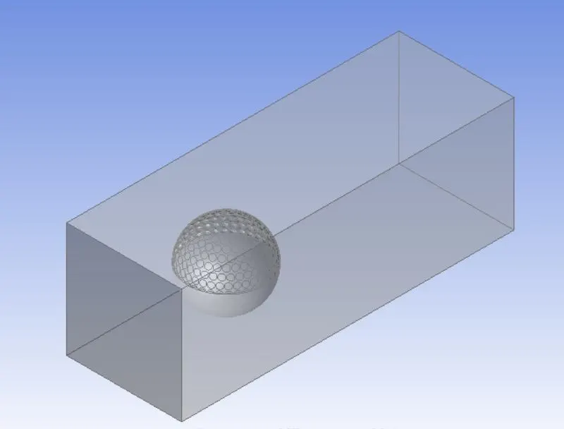
• Then using the slice command select the required plane >> click apply >> Generate. Now, the single solid body is converted into 2 solid bodies.

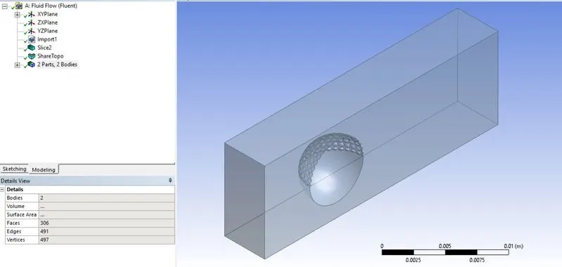
• Select the body which is not necessary >> Right click mouse >> Suppress the solid body. The model is now split from mid-section, as result with less no. of mesh element & computational time we can obtain the same result.

Mesh:

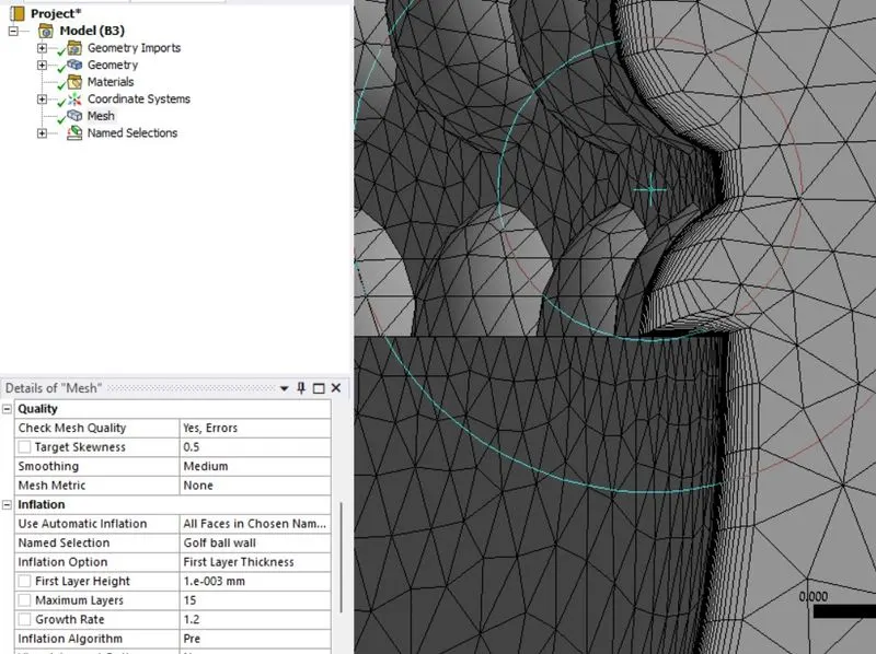
• Mesh >> Element Size 0.5mm, Target Skewness 0.5, Inflation First Layer Height Is 0.001mm, 15 Layers, 1.2 Growth Factor >> Generate.

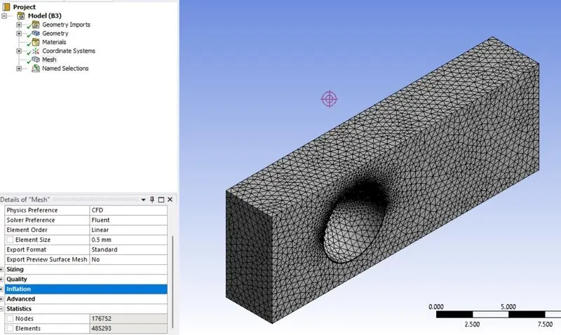
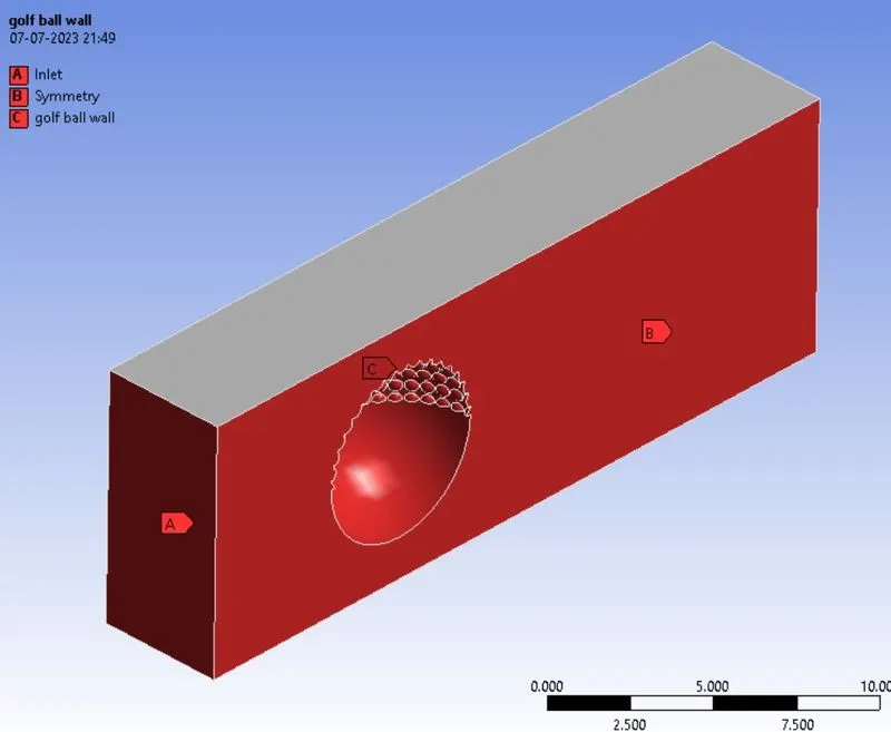
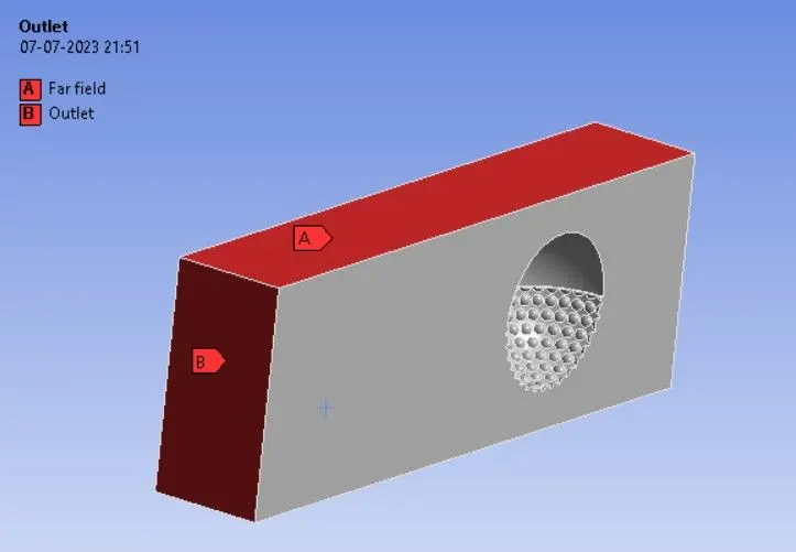
• Select the faces and name them.

Setup:

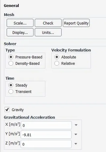
• General setting >> Pressure based solver >> Absolute >> Steady state simulation. As the flow is below 0.3 Mach no. hence pressure-based solver is used.

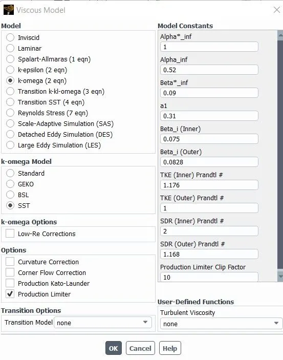
• Viscous model >> K-Omega model SST model
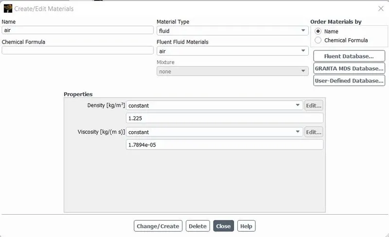
• Material: Air

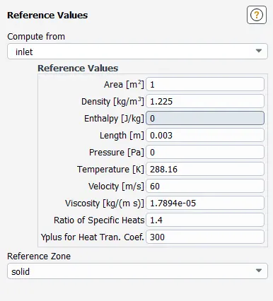
• Reference values

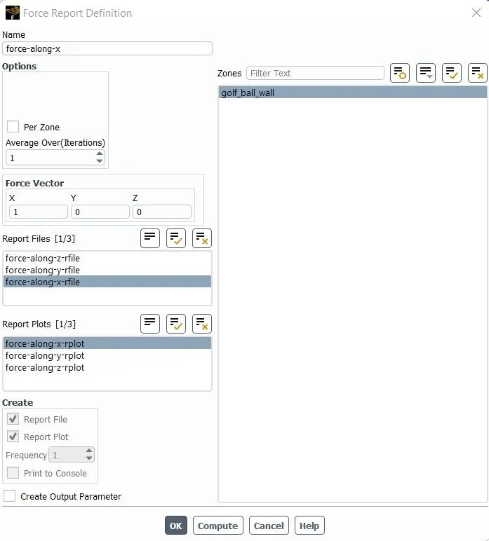
• Report Definition

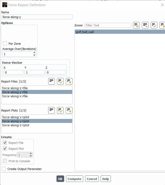
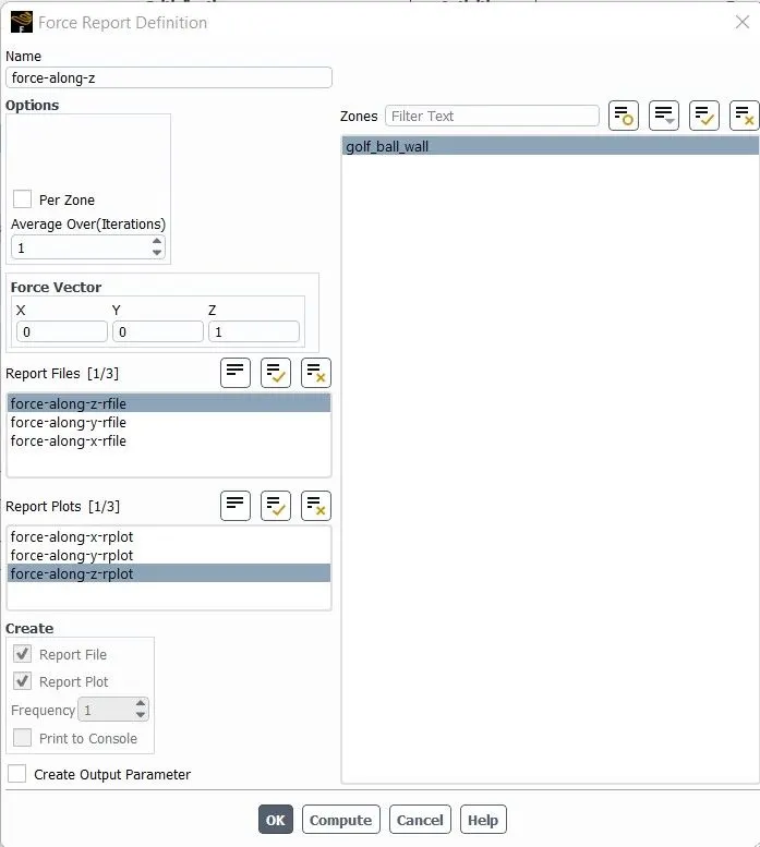
Solution:

• Residual

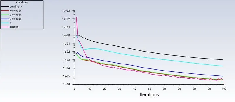
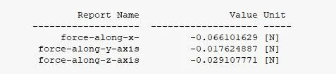
• Force along X axis plot

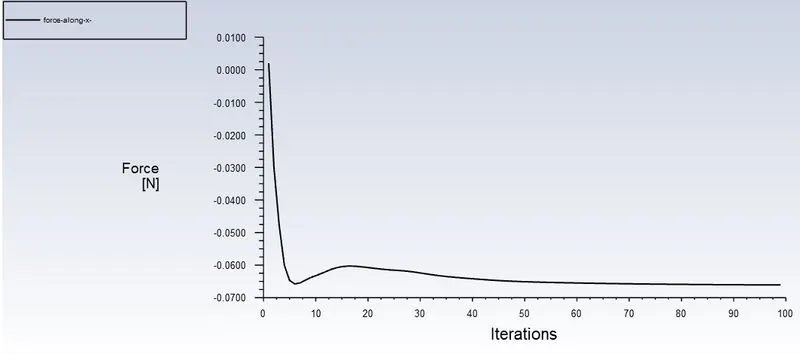
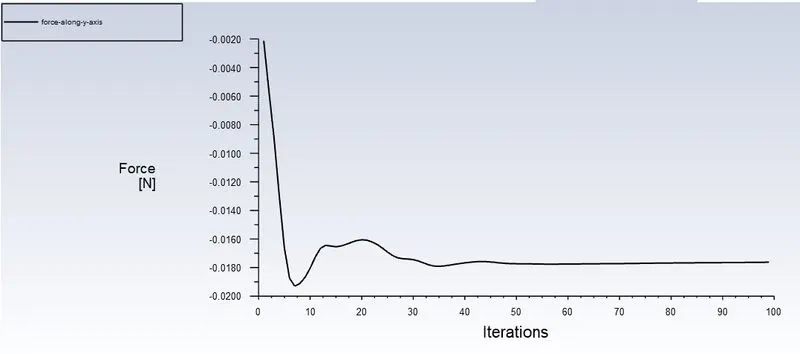
• Force along Y axis plot

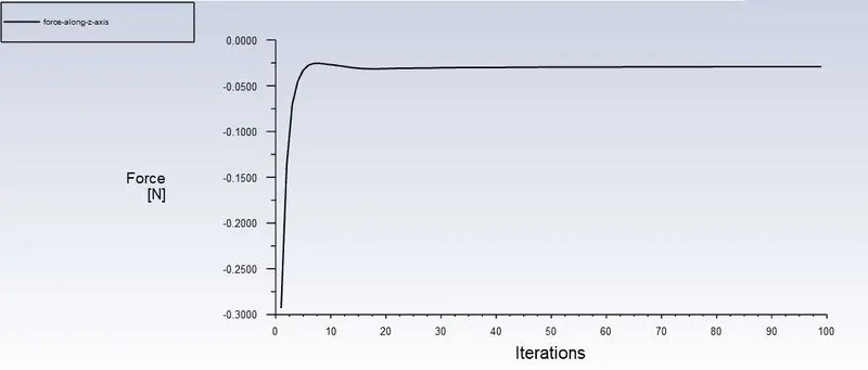
• Force along Z axis plot

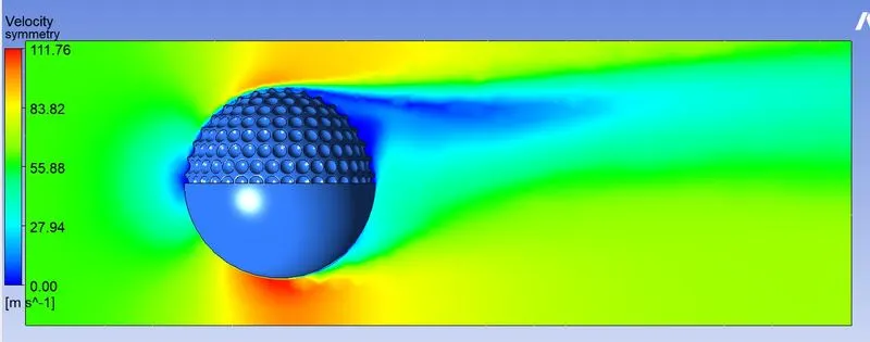
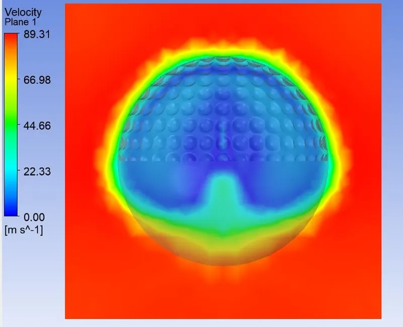
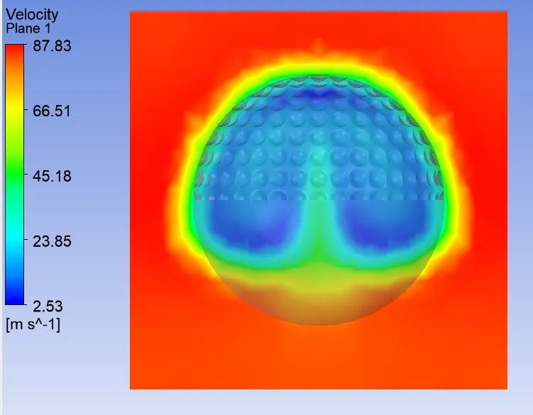
• Velocity Contour

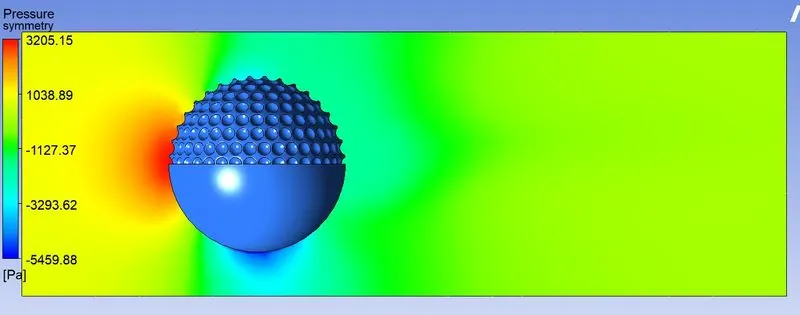
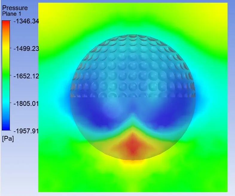
• Pressure Contour

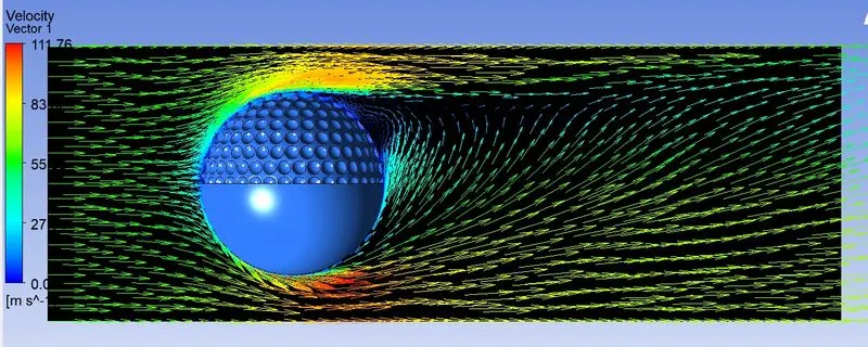
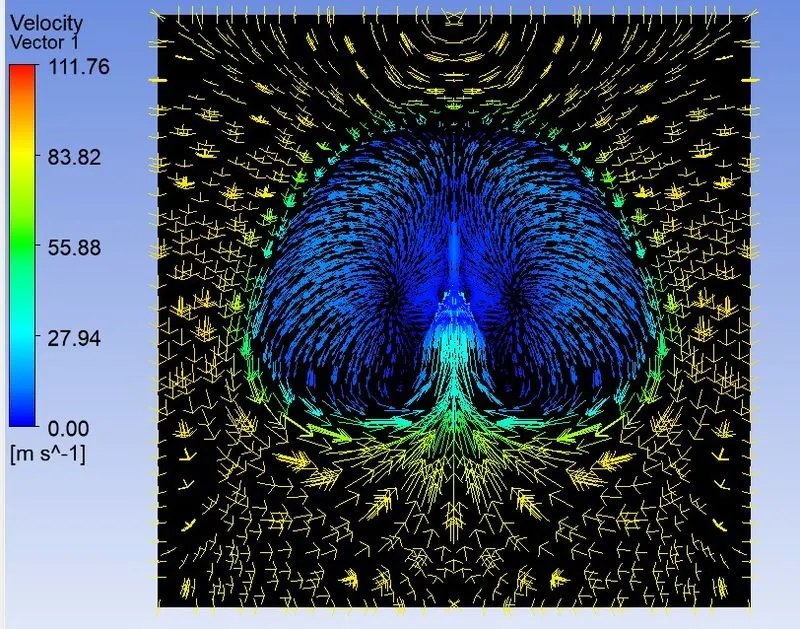
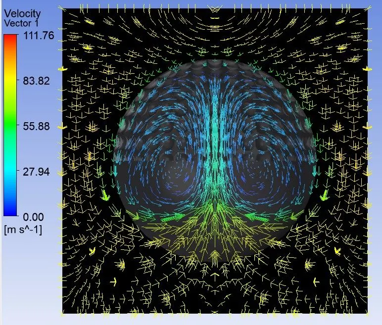
• Velocity Vector

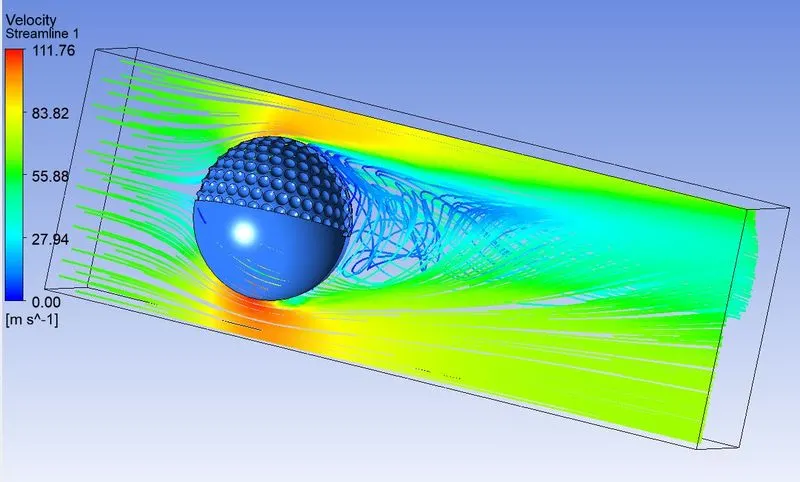
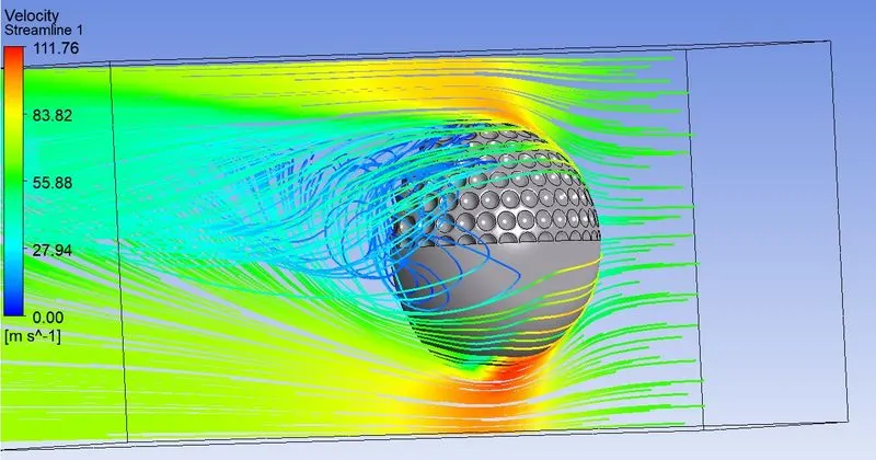
• Streamline plot

Result:

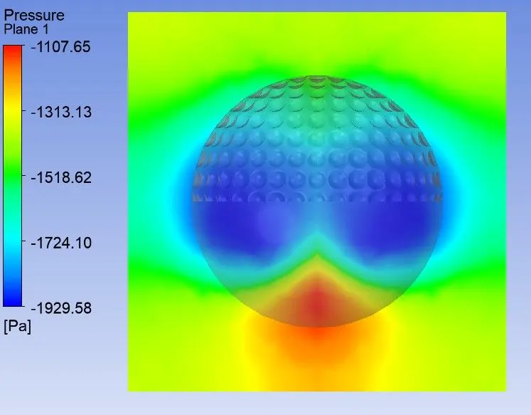
• Midplane of golf ball

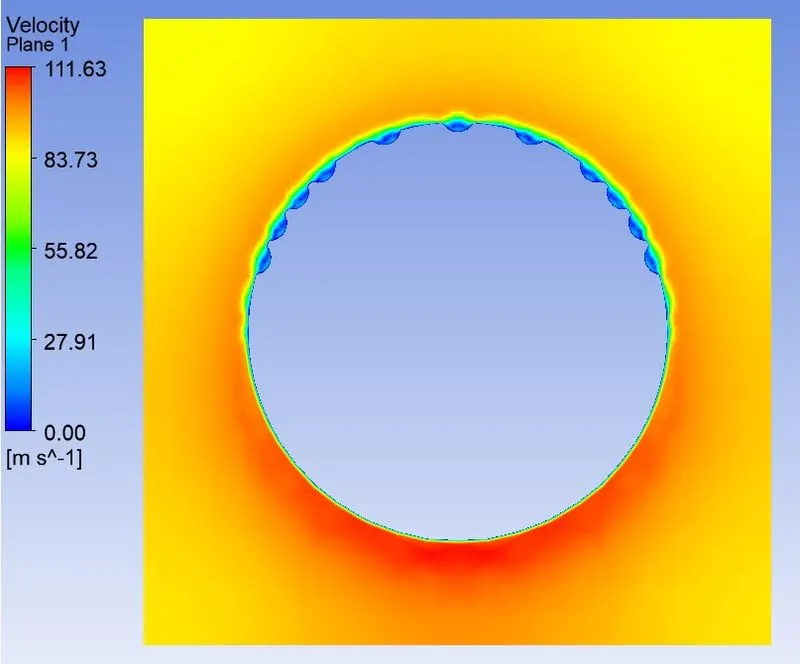
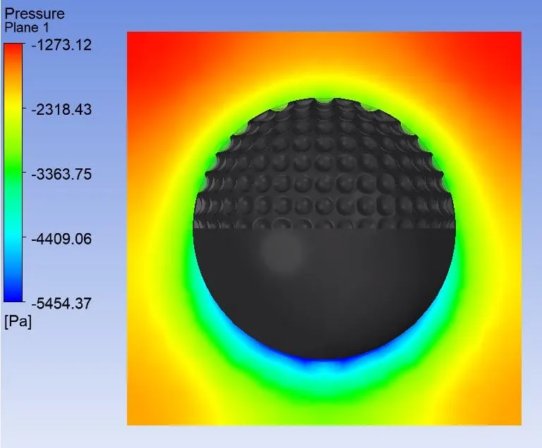
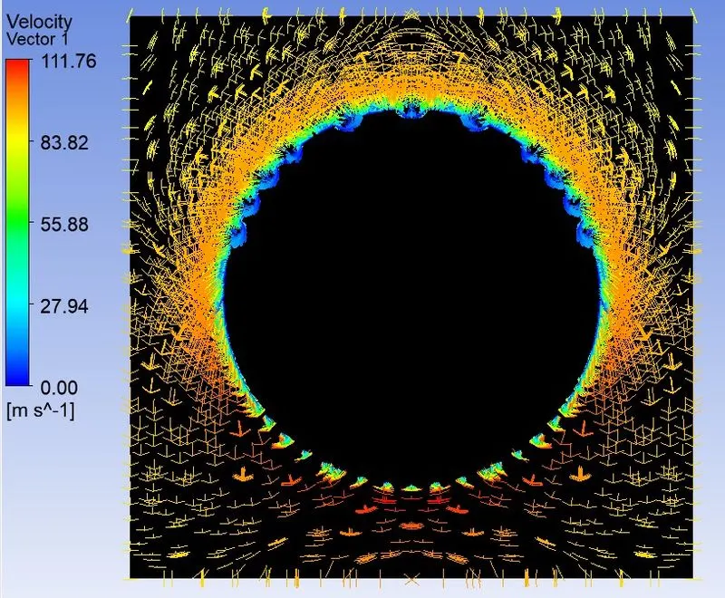
• 0.001mm from midplane towards the trailing side

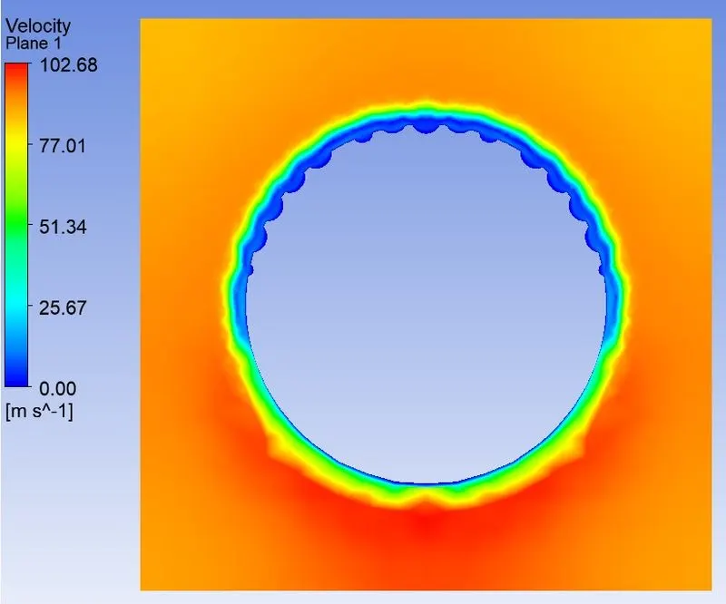
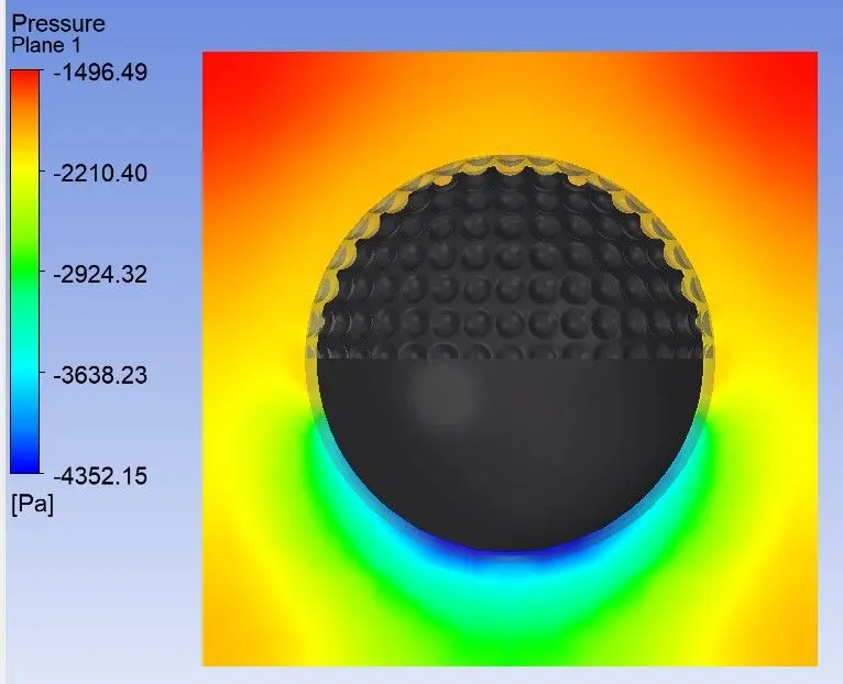
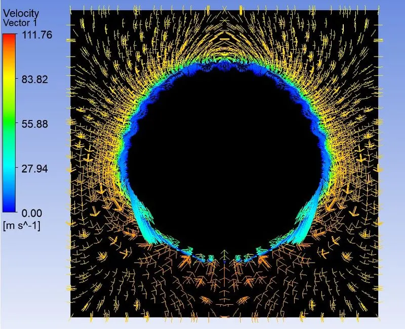
• 0.002mm from midplane towards the trailing side

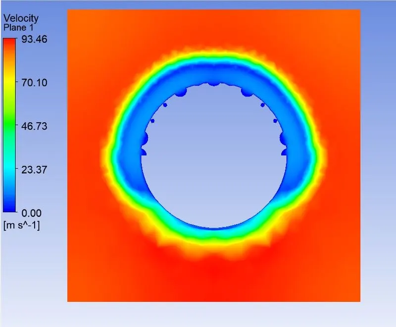
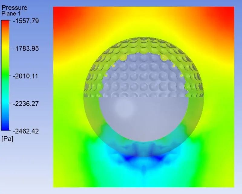
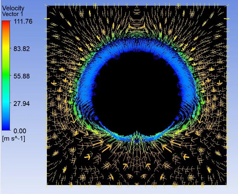
• 0.003mm from midplane towards the trailing side

• 0.004mm from midplane towards the trailing side

Conclusion:

• Resultant forces acting on Golf Ball

• From the pressure contour it is found that the low pressure zone is found at the smooth side & high pressure zone is found at the dimple side, as a result of pressure differential the ball is projected downwards.
• When the air flows around the smooth surface it gets detached early as compared to the dimple side, this is because the air flowing through the dimples the air becomes turbulent and creates the low pressure zone and sucks the air flows and helps it attach to the surface.
• It is said that the dimpled golf ball travels twices the distance as that of the smoothed ball, this is possible only due to reduced wake region at the trailing side of the dimpled golf ball as compared to the smoothed surface ball. The wake produced behind the ball creates a low pressure zone which inturn sucks the ball in the opposite direction thus reducing the ball speed.
• From the current simulation it can also be seen that low pressure zone created at the trailing side of the smooth surface is larger as compared to the low pressure zone created at the dimple side which justifies our previous points.