Week 5 - Turbulence modelling challenge

Turbulence modelling challenge

Aim:To perform turbulence modelling of golf ball.

Objectives:

1. To do a literature review of various turbulence models explained in the Turbulence modeling video (Week-5) and explain why DNS isn’t feasible according to Kolmogorov's scale.
2. For the below geometry performs a 3D simulation and explain the recirculation region using velocity vectors.
3. Consider the flow direction of air, the ball is traveling opposite to it at 60m/s. Explain in which direction the ball will curve by visualizing the wake region.

Theory:

Turbulence models in Computational Fluid Dynamics (CFD) are methods to include the effect of turbulence in the simulation of fluid flows. The majority of simulations require a turbulence model as turbulent flows are prevalent in nature and in industrial flows and occur in most engineering applications.

Turbulence is the apparent chaotic motion of fluid flows. Fluid flows can be laminar, when they are regular and flow in an orderly manner. When the speed or characteristic length of the flow is increased, the convective forces in the flow overcome the viscous forces of the fluid and the laminar flow transitions into a turbulent one. The ratio between convective and viscous forces is called the Reynolds number. This number can be used to classify the type of flows, the higher the number the more turbulent the flow is.

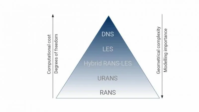
Most of the time, in engineering applications we interested in mean or integral quantities like forces on a body or mass flow rate through a passage. In order to obtain such quantities, solving turbulent flows with a turbulence model is not only sufficient, but recommend too, as in this way it is possible to obtain reliable solutions in a more efficient and cost effective way. The figure below shows a summary of the most common approaches to solve turbulent flows. The computational cost a CFD simulation increases from RANS to DNS as the number of degrees of freedom required to solve the flow increases. As a consequence of the computational cost, scale resolving approaches like DNS and LES are generally applied to simple geometries and academic configurations, while hybrid RANS-LES, URANS and RANS can be applied to complex industrial problems.

The turbulent models are as follows, in order of
increasing complexity:
ƒ Algebraic (zero equation) mode : mixing length (first order ls model)
ƒ One equation models: k‐model, μt‐model (first order model)
ƒ Two equation models: k‐ε, k‐kl, k‐ω2, low Re k‐ε (first order model)
ƒ Algebraic stress models: ASM (second order model)
ƒ Reynolds stress models: RSM (second order model)

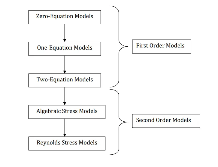
First order models are based on the analogy between laminar and turbulent flow.They are also called Eddy Viscosity Models (EVM). The idea is that the average turbulent flow field is similar to the corresponding laminar flow.

In zero equation models, as the name designates, we have no PDE that describes the transport of the turbulent stresses and fluxes. A simple algebraic relation is used to close the problem. Based on the mixing length theory, which is the length over
which there is high interaction of vortices in a turbulent flow field.

In one‐equation models, a PDE is derived for the turbulent kinetic energy and the unknowns (turbulent viscosity and conduction coefficient) are expressed as a function of the turbulent kinetic energy.

In the two‐equation models, we develop two PDEs: one for the turbulent kinetic energy and one for the turbulent dissipation rate.The idea is to express the turbulent viscosity as a function of K and ε and then derive PDEs for K and ε.

The central concept of second order models is to make direct use of the governing equations for the second order moments (Reynolds stresses and turbulent fluxes) instead of the questionable Boussinesq hypothesis. The motivation is to overcome
the limitations of first order models in dealing with the isotropy of turbulence and the extra strains. The overshoot of this approach is the large number of PDEs induced which involve many unknown or impossible to find correlations. The most
famous models are the Algebraic Stress Model (ASM) and the Reynolds Stress Model (RSM).

DNS isn’t feasible according to Kolmogorov's scale:

DNS creats a very small mesh and tries to capture all cells.It is not possible to perform DNS simulation in Fluent because of the fact that DNS requires too much computational effort.

Procedure :

• Import geomtry in design modeller and generate the geometry.

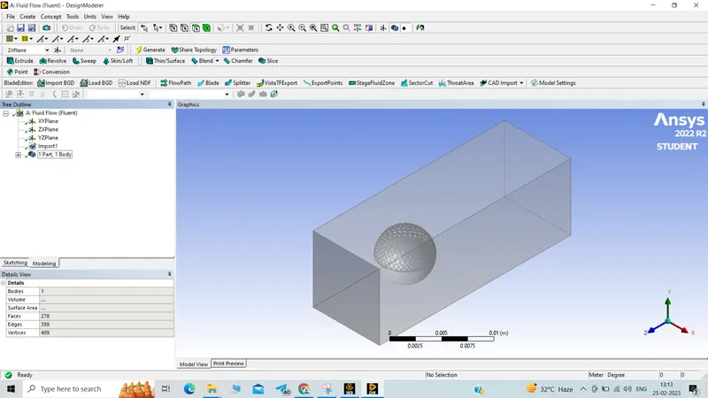
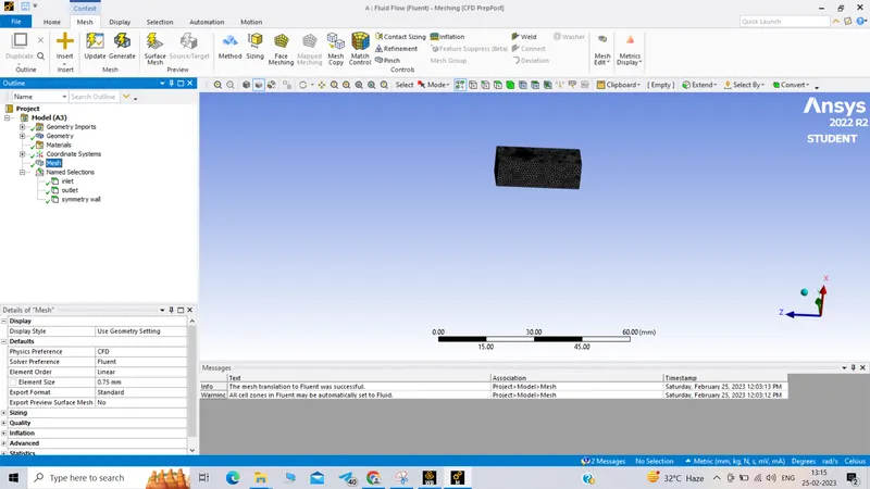
• Perform meshing with base mesh then refined with decreasing size of element.

Create named selction

• Set up:

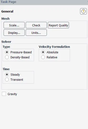
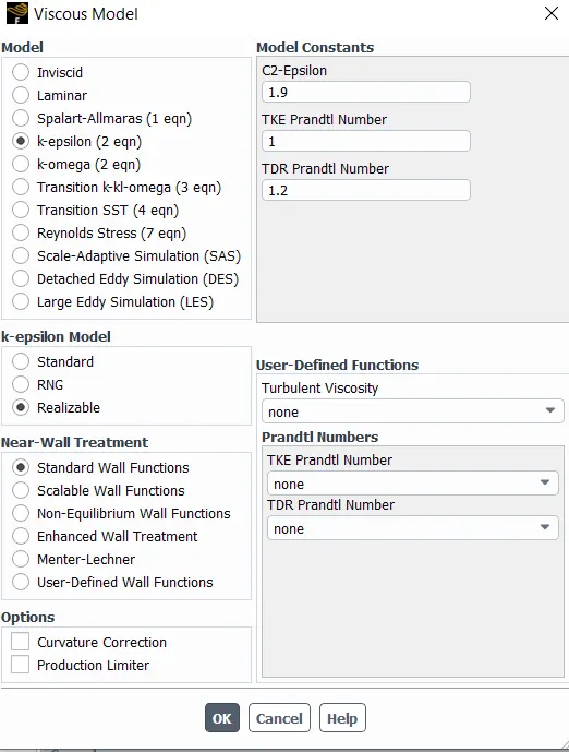
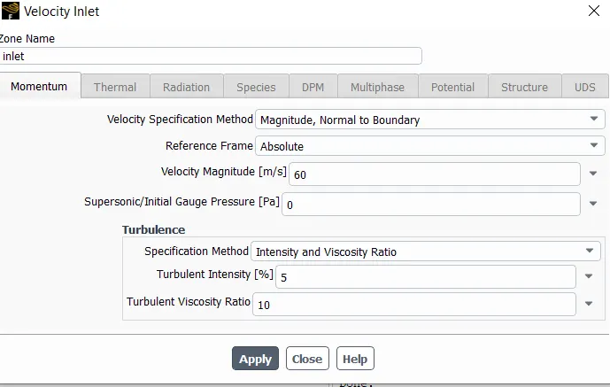
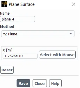
• Solution:

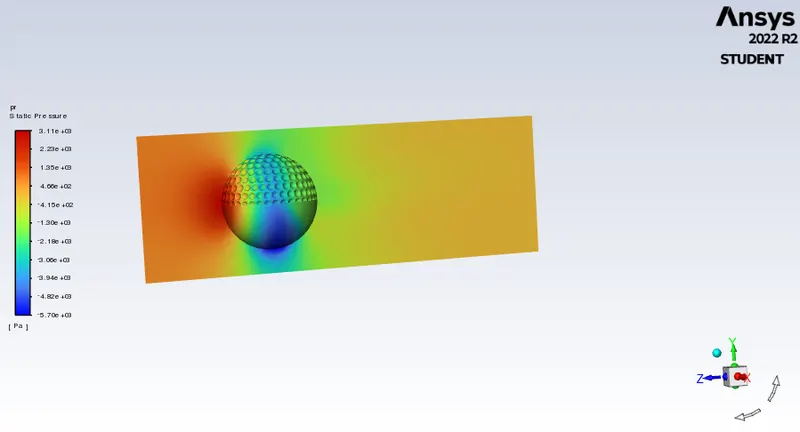
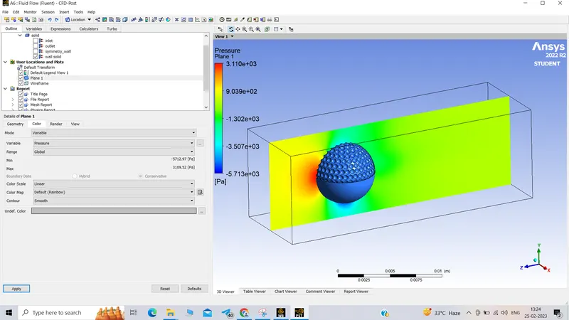
Pressure contour at plane:

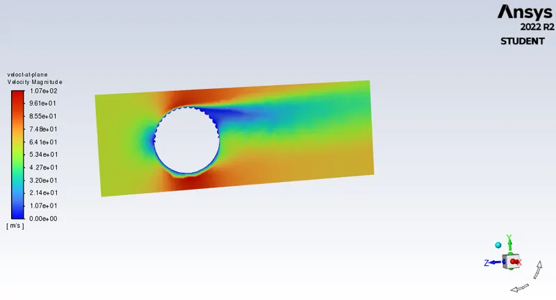
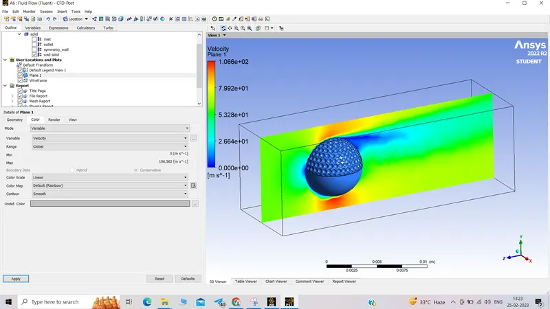
Velocity contour at plane:

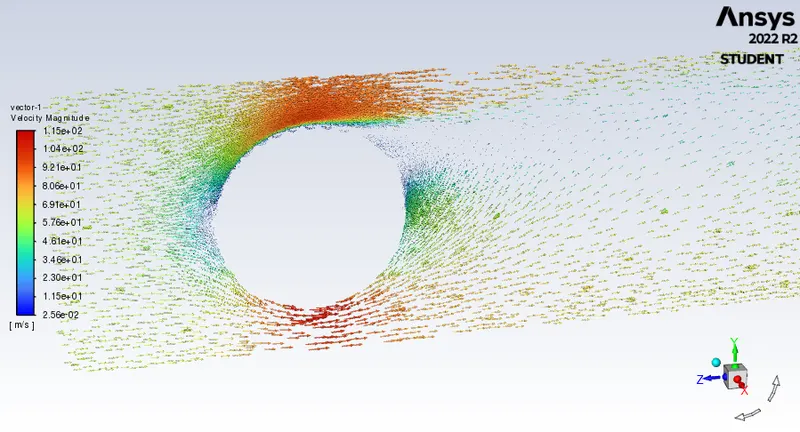
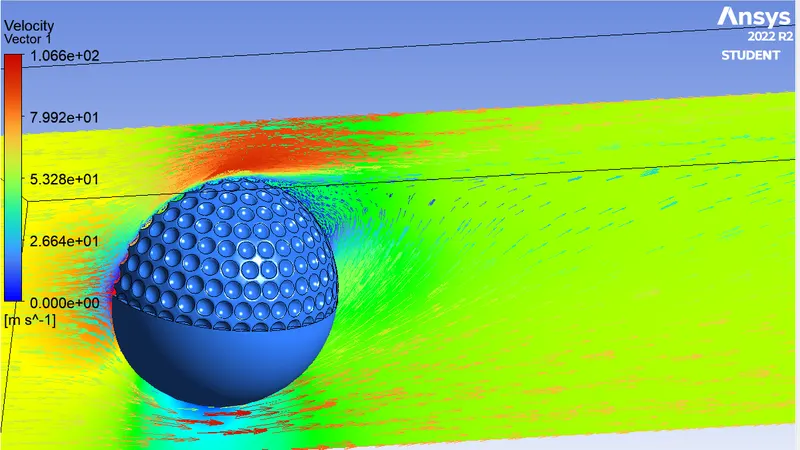
Velocity vector contour:

Result:

The golf is moving down as the velocity is high under the ball hence pr is low and on the upper side the velocityis high hence pr is high.So there is a difference in pr and the ball is moving down.The wake region or recirculation region at the back side of ball shows the direction of arrow circulating downward. The recirculation region also helps the flow seperation from the ball.

The dimple in tha ball induce turbulence and delay flow seperation hence reduce drag force.