Week 5 - Turbulence modelling challenge

Aim- To understand and simulate the turbulence flow over the Golf ball and find in which direction the ball will curve by visualizing the wake region.

To understand turbulence let's first understand the Reynolds number because the Reynolds number helps us to define the point of turbulence of a fluid flow. By the help of the Reynolds number, we can say whether the fluid flow is laminar or turbulent flow. Then we will try to understand why DNS isn't feasible according to Kolmogorov's Scale.

Reynolds Number-

Reynolds number is a dimensionless quantity Which is used to determine the type of flow pattern as laminar or turbulent. Reynolds number is defined as the ratio of inertial forces to that of viscous forces.

Where,

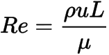
Re is the Reynolds number

ρ is the density of the fluid (kg/m3)

V is the velocity of flow (m/s)

D is the pipe diameter (m)

μ is the viscosity of the fluid (kg/m.s)

The Reynolds Number can be used to determine if the flow is laminar, transient or turbulent. The flow is

laminar - when Re < 2300

transient - when 2300 < Re < 4000

turbulent - when Re > 4000

Turbulence Model- Turbulence is that state of fluid motion which is characterized by apparently random and chaotic three-dimensional vorticity. When turbulence is present, it usually dominates all other flow phenomena and results in increased energy dissipation, mixing, heat transfer, and drag. If there is no three-dimensional vorticity, there is no real turbulence.

First-Order Models: Because the PDEs used to solve the turbulence in these models are of the first order, they are referred to as first-order models. This presupposes that laminar and turbulent flows are analogous. In comparison to second-order models, the average turbulent flow field is comparable to equivalent laminar flow. These models are best suited for satisfactory results with less processing power and less expense. These are commonly employed to tackle problems with turbulent viscosity.

Types of Computational Approach

DNS - Direct Numerical Simulation

LES - Large Eddy simulation

RANS - Reynolds Averaged Navier stokes simulation

Direct Numerical Simulation (DNS) involves the direct solution of the unsteady N–S equations, and are thought to be capable of resolving even the smallest eddies and time scales of turbulence within a flow. Although the DNS method does not require any additional closure equations very fine grids and extremely small time steps need to be used, in order to obtain accurate solutions. This method is currently confined to simple flow problems at relatively low Reynolds numbers. DNS computations of the fully turbulent high Reynolds number flows associated with ship flows await major advances in computational hardware. Although DNS solvers are limited to solving low Reynolds flows.

Large Eddy Simulations (LES) is a cutting-edge technique that is used to simulate how hardware interacts with fluids. It strikes a balance between computational efficiency and granularity, which has led to tremendous popularity in the aerospace and automobile industry. The main computational benefit comes from filtering, which chunks our data into computationally feasible blocks. For information in each block, we directly solve the equations and for smaller Sub-Grid Scale (SGS) data.

Reynolds Average Navier Stokes simulation (RANS)-

• Solves Time - Averaged Navier stokes equation
• All turbulent motion is modelled
• For most problems, the time-averaged flow (and level of turbulence) are all that is needed
• Many different models are available
• This is the most widely used approach for industrial flows

The RANS-based simulation consists of two types of equation models-

1. One Equation model

• Spalart-Allamaras Model-

  The Spalart–Allmaras model is a one-equation model that solves a modelled transport equation for the kinematic eddy turbulent viscosity. In its original form, the model is effectively a low-Reynolds number model, requiring the viscosity-affected region of the boundary layer to be properly resolved ( y+ ~1 meshes).The Spalart–Allmaras model was developed for aerodynamic flows. It is not calibrated for general industrial flows and does produce relatively larger errors for some free shear flows, especially plane and round jet flows. Incorrect for Shear flow, Separated Flow, or decaying TurbulenceIt solves a transport equation for a viscosity-like variable. This is called the Spalart–Allmaras variable.

2. Two Equation model

• K-epsilon Model

1. Standard K-epsilon (k-ε)-turbulence model is the most common model used in CFD to simulate mean flow characteristics for trubulant flow conditions. It is a two equation model that gives a general description of turbulance by means of two transport equations (PDEs).It is suitable for free-shear layer flows with small P gradients and It uses wall functions to calculate epsilon near wall. It consumes low memory requirements and stable outcomes. The first transported variable is the turbulent kinetic energy (k) and second transported variable is the rate of dissipation of turbulent kinetic energy (ε). It is inaccurate for adverse pressure gradients, strong curvature, and jet flow but valid only for fully turbulent flow.

2. Realizable K-epsilon model- The modified epsilon equation model is a realizable k-epsilon model. It also shows higher performance for flows including rotation, boundary layers under significant unfavorable pressure gradients, separation, and recirculation when compared to turbulent models. In almost every comparison, Realizable k-€ outperforms the competition in terms of capturing the mean flow of complicated structures.
3. Renormalized Group(RNG) model- It features a much-enhanced epsilon equation that includes whirling effect modeling. It finds a modified version of Prandtl Number using empirical relations. It is favourable for indoor air flow simulation. It is inaccurate for vortex-free evolution and also unstable with steady state solutions. It consumes 10-15% more CPU time then other two -epsilon Model.

• K-Omega Model-The K-omega model is one of the most widely utilized in the business. The RANS model includes this model (Reynolds averaged Navier stokes equation)

1. Standard k-omega model: The standard model is a low model that may be employed for low Reynolds number flows with a relatively thick boundary layer and a viscous sublayer that can be resolved. As a result, for near-wall treatment, the conventional model is optimal. Improved performance for complicated boundary layer flows under unfavourable pressure gradients and separations is another benefit.
2. SST k-omega model: Shear stress transfer k-omega model (SST k-omega model). It's a better variant of the traditional k-omega model. It's the most common model for modelling near the wall and away from the wall, and it's the most popular model for modelling near the wall and away from the wall. Transitions from a standard model to a high Reynolds model away from the wall using a mixing technique.

Second-Order Models:

Solves transport equations for Reynolds stress terms using second-order models. These models are the most precise and are most sensitive to boundary conditions. They're also time-consuming to compute.

Algebraic Stress Model: The algebraic Reynolds stress model is derived from the Reynolds stress dynamic equations.

Reynolds Stress model: In inflows with high degrees of anisotropy, considerable streamline curvature, flow separation, zones of recirculating flow, or flows impacted by rotational forces, the Reynolds Stress model RM provides superior accuracy than k-omega and k epsilon.

Turbulence on the Kolmogorov scale: Advanced theoretical fluid dynamics may be used to determine the smallest sizes of turbulence. Turbulent kinetic energy is transferred from bigger eddies to smaller eddies in the cascade process.

According to universal equilibrium theory, smaller eddies should absorb energy from bigger eddies and disperse it in about equal amounts as heat and acoustic radiation. Small scale motion is mostly determined by which bigger eddies provide energy, and

kinematic viscosity is equal to = dK/dt

Why DNS isn’t feasible according to Kolmogorov's scale?

When a fluid is in a turbulent flow regime, i.e. when the flow around the body surpasses critical velocity, bigger eddies break into smaller eddies, and sometimes smaller eddies combine to form larger eddies. Energy cascading is the term for this process.

We can't utilize DNS since it creates a very small mesh and tries to capture all anomalies (cells), therefore as the number of mesh cells grows, the time it takes to solve grows. As a result, industries dislike this strategy.

Part-2

Geometry-

Import Geometry of the golf ball with enclosure into the Design Modular of Ansys Workbench

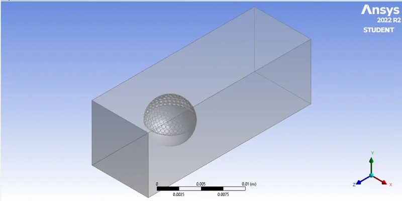
Mesh-

Named the edges using Named selection option in mesh- Inlet, outlet, walls

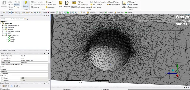
Generate a mesh

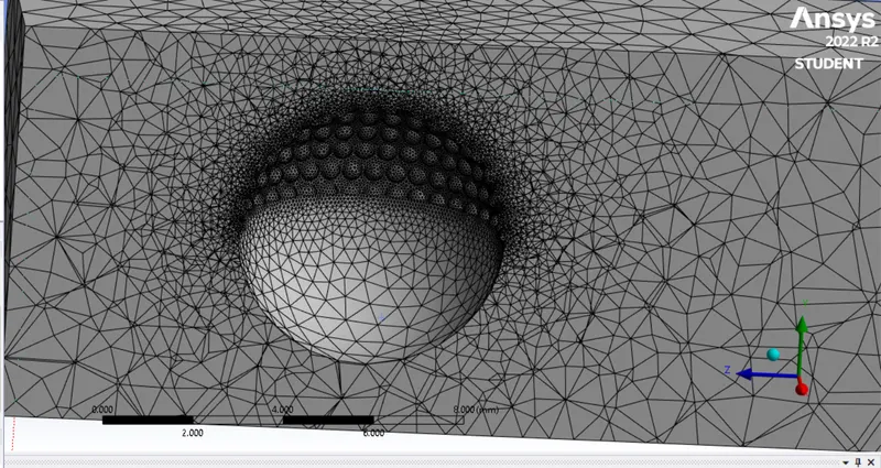
We are going with base line mesh because of the limitations of the learning license of the Ansys fluent.

Setup-

For this simulation, we go with-

Steady-state simulation

Velocity formulation as Absolute

Pressure Based simulation

Boundary conditions

Inlet- 60m/s

Outlet- 0 pascal

Walls- walls

We will go with Hybrid Initialization.

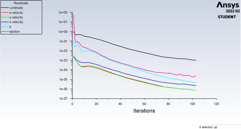
We ran this simulation for 250 iterations. but it got converged on the 110th iteration.

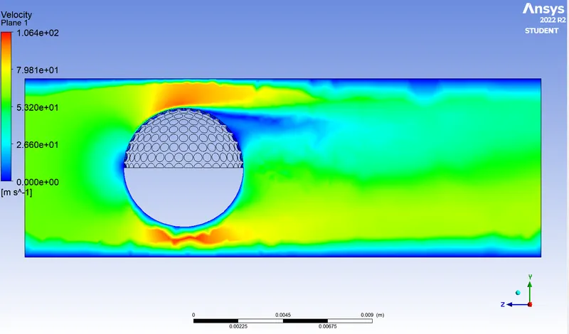
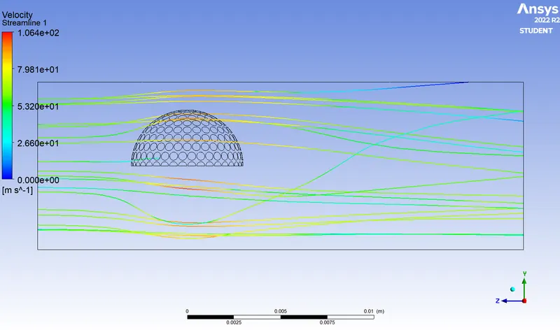
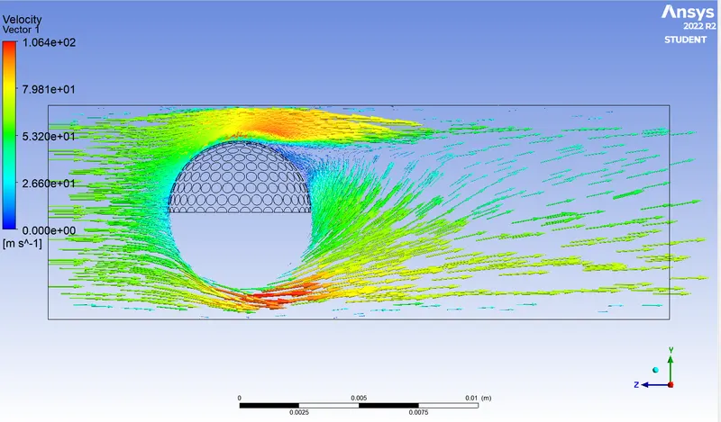
As We can identify the direction of the ball by looking at the velocity vectors and claim it's moving down. In an anti-clockwise direction.

Wake Region- The Wake region is formed by turbulence which originates in the flow region with highest velocity gradient and by the coalescence of the free shear layer shed from the body surface when the boundary layer leaves the surface.

The golf ball's dimples serve to minimize drag by minimizing the wake region.It also aids in the attachment of the flow and attempts to detach the flow from the golf ball.

Therefore The velocity of the flow beneath the golf ball is high, resulting in low pressure and the formation of a wake following the rough surface. The air velocity on the rough surface is lower, whereas the air velocity on the smooth surface is higher. This causes a pressure differential, which accounts for the ball's downward swing.