Week 5 - Turbulence modelling challenge

Turbulance Models

Spart Allmaras

the Spalart–Allmaras model is a one-equation model that solves a modelled transport equation for the kinematic eddy turbulant viscosity. The Spalart–Allmaras model was designed specifically for aerospace applications involving wall-bounded flows and has been shown to give good results for boundary layers subjected to adverse pressure gradients. It is also gaining popularity in turbomachinary applications.

In its original form, the model is effectively a low-Reynolds number model, requiring the viscosity-affected region of the boundary layer to be properly resolved ( y+ ~1 meshes). The Spalart–Allmaras model was developed for aerodynamic flows. It is not calibrated for general industrial flows, and does produce relatively larger errors for some free shear flows, especially plane and round jet flows. In addition, it cannot be relied on to predict the decay of homogeneous, isotropic turbulence.

It solves a transport equation for a viscosity-like variable . This may be referred to as the Spalart–Allmaras variable.

K-epsilon Model

K-epsilon (k-ε) turbulence model is the most common model used in CFD to simulate mean flow characteristics for trubulant flow conditions. It is a two equation model that gives a general description of turbulance by means of two transport equations (PDEs). The original impetus for the K-epsilon model was to improve the mixing length model, as well as to find an alternative to algebraically prescribing turbulent length scales in moderate to high complexity flows.

• The first transported variable is the turbulent kinetic energy (k).
• The second transported variable is the rate of dissipation of turbulent kinetic energy (ε).

• Standard K-epsilon model

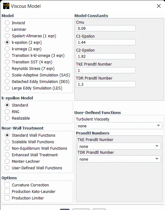
This model is most widely used in industies since they are known for its good convegance and memory efficiency. They use wall function to calculate near wall. Good for attached and turbulance flows also for flow around complex geometries. However they are not good for sperated flows

• Realizable K-epsilon model

• Renormalized Group(RNG) model

K-omega model

The K-omega model is one of the most commonly used turbulance models. It is a two equation model, that means, it includes two extra transport equations to represent the turbulent properties of the flow. This allows a two equation model to account for history effects like convection and diffusion of turbulent energy.

The first transported variable is turbulent kinetic energy, . The second transported variable in this case is the specific dissipation, . It is the variable that determines the scale of the turbulence, whereas the first variable, , determines the energy in the turbulence.

• Standard k-omega model
• SST k-omega model

why DNS isn’t feasible according to Kolmogorov's scale

• More time needed to converge
• Very fine meshes which results in more computational resources needed to run Hence industries dont preffer this method as its inefficient

Simulation

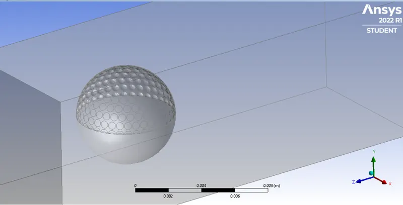
Geometry

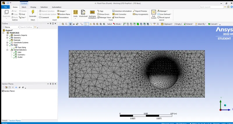
Mesh

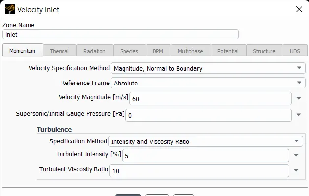
Setup

Results

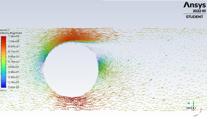
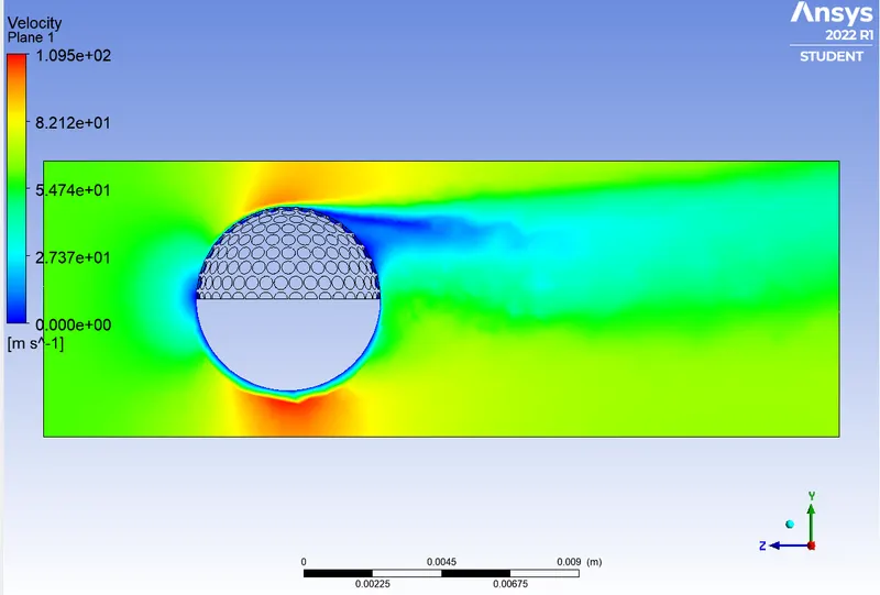
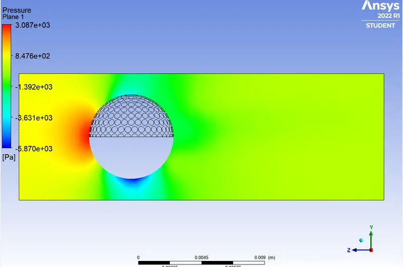
• The dimples have significant effect on drag as it reduces the wake region
• Usually this design is used by golf ball so to increase the range and accuracy of the shot
• By looking at the contours we can conclude that the ball moving down as it progresses throgh air

Conclusions

• Done a literature review of Turbulance models
• Simulated an external flow around a sphere with dimples
• Extracted contours