Week 5 - Turbulence modelling challenge

Literature review of Turbulance Model

Turbulance modelling has been an area of research for long. As the research has progressed various models have been introduced that have been able to model turbulance computationaly. Although, the accuracy has been subjective there are models that the industry has been employing for long.

The turbulance models can be categorised on the basis of equations they employ as:

1. Zero equation model: In these models the Velocity scale and the length scale is calculaed from the local mean flow. This kind of models are used to validate the flow whilst a more complex modlling is done. For complex flows this is not a good model as it does not capture the turbulance correctly. Also, in complex flows the distribution of the mixing lengths is rapidly changing. Since, the mixing lengths are constant in this model it is unfeisible to use it for complex flows. 

But, being an simple model it is computationally economical and suitable for simple shear-layer-dominated or pressure-drive-flows. 

The Models that are based on this are:

1) Constant viscosity model

2) Prandlt Mixing-Length model

3) Lvel Turbulance model (Good for electronic equipment where the grid is coarse for 2 equation models)

2. One equation model: In this type, one of the Velocity is evaluated using an equation and the lengthscale is evaluated using an emperical relation. 

As the velocity is prescribed using an equation. Since, the length scale is rigid and not able to change because of this it is not good for flow separation anallysis hence a 2 equation approach is used.

Spalart–Allmaras model is a One equation model ideally for the aerospace indusrt and performs bad with industrial applications.

3. Two equation model:  

In this form of modelling 2 extra PDE are introduces to understand the turbulance. These are used to evaluate the Turbulance kinetic energy and dissipation. Since 2 extra PDE are introduces it becomes computationally heavier than the Mixing length models.

a) k-`epsilon` Model: 

Turbulance Kinetic energy: 

Turbulance Dissipation:

The constant are experimentally derived and are based on various turbulance flows.

This is a widely used model for the induatrial and environmental applications. It is robust to the initial and boundary condition. This model is perticularly well suited for shear flows and recirculating flows. 

As it is holds its ground for the lower pressure gradients it is not well suited for adverse pressure grdients and by association flow separation. 

b) k-`omega` Model:

the k and `omega` is model based on the equation above.

As this is a low Re model which has bigger boundary hence the viscous layer can be resolved easiely. This model's performance for the better near wall treatment this gives it a better ability to handle adverse pressure gradient and by association better flow separation prediction. In these regards the k-omega is better than the k-epsilon model.

The 2 equation models mentioned above are also known as RANS - Reynolds Averaged Navier-Stokes model. 

Bases on these models further models have been developed which cater to various applications such as k-epsilon (RNG), K-omega (SST).

The following simulation is conducted in asys fluent.

The model used is k-omega standard. With velocity inlet of 60m/s. For convinience to stay in the number of cell limit the body is split in the middle ane that wall is considered as a symmetry wall. 

The contours of the simulation is as shown

Pressure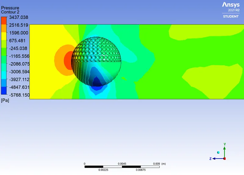
Velocity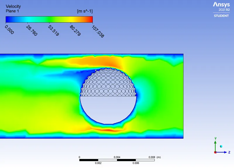
Velocity (vector plot)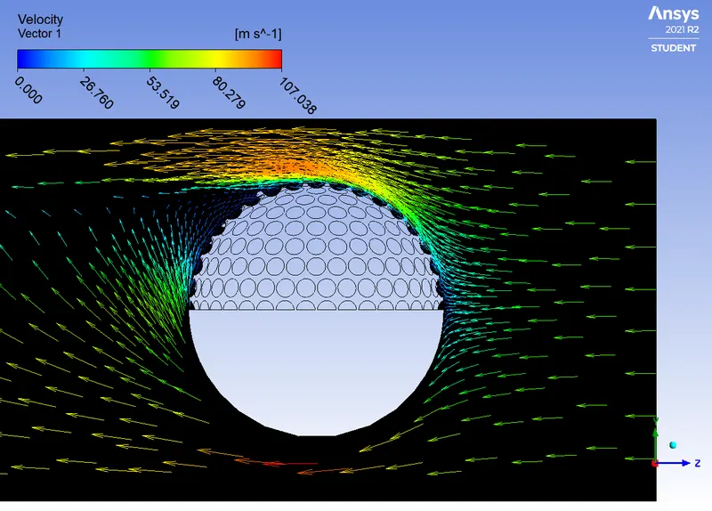

From these contours and velocity profile we can see that at the top part the pressure distribution is more evenly distributed which means the generation of adverse pressure gradient developed later than the bottom part. Hence, the flow separation takes place later which improves the aerodynamic performance of the ball. 

Because the lower pressure is devloped on the smoother side this gives rise to the pressure drag and since the adverse pressure gradient is developed the flow separation takes place. 

Although, the pressure gradient is developed on both the sides, on the top side the point so separation is further back from the smooth part. Flow separation is bad in this case as it might influence the trajectory of the ball, these dimples are what keep the flow from developing the boundary and lead to an adverse pressure gradient which smooths out the pressure on the whole surface of the ball.