Week 4 - CHT Analysis on Exhaust port

Introduction: Conjugate heat transfer analysis is a computational method which involves analyzing heat transfer from fluid to solid and vise-vers. Here extra Enegry equation is needed to be solved besides Navier-Stokes equation. There are various applications for CHT from understanding the effects of thermal stresses on the components of an engine, to understanding the cooling of an elctronic appliances. CHT is essential for engineering applications as it helps optimize the design which would result in efficient use heat and thermal energy or its removal from the system.

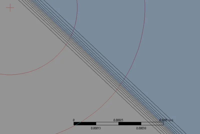
As heat transfer takes place from fluid to solid in this case, it is crucial to understad and have a correct value of heat transfer coeffiient. This can be calculated colse to the solid wall, Due to the tetrahydra mesh the cells close to wall are not as perfect and they often cause diffusion and inaccurate. To avert this problem y+ (a non-dimentionless number) is used to calculate the first wall thickness and it should be close to the wall boundary. In the current case using the formula for y+

`y+ = (y*ut)/ nu`

Using the current case y+ of ariound 5 mm is used. 

 It is important to keep the y+ value in accordance with the turbulance model used. As some models are suited for resolving of near wall physics such as k-Omega (SST) a y+ of approx. 1 is considerd to be good, where as the y+ for k-Epsillon ranges from 30 to 300. 

The case setup has been set using 3 cases:

1) base case (k-epsillon) without inflation layer

2) k-Episillon with inflation layers

3) k-Omega with inflation layers.

 Problem setp:

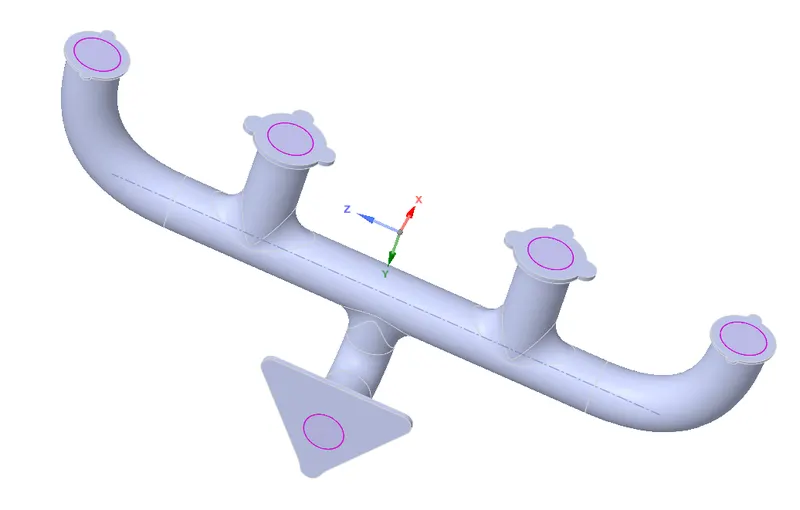
Geometry:

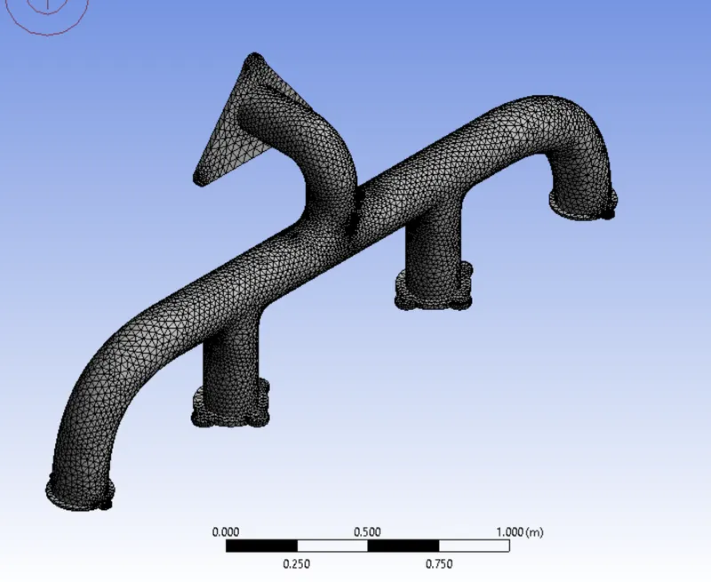
Mesh:

Inflation layer

Case setup:

As studies conducted involved both k-Omega (SST) and k-Epsillon. Energy is turned on for this simulation as there is heat trasfer with the fow as well.

The boundary conditios are initiated with velocity of 5m/s

 The results and post-processing files are mentioned below:

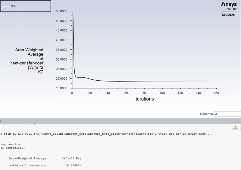
Case 1 Without inflation
Case 2 k-Epsilon
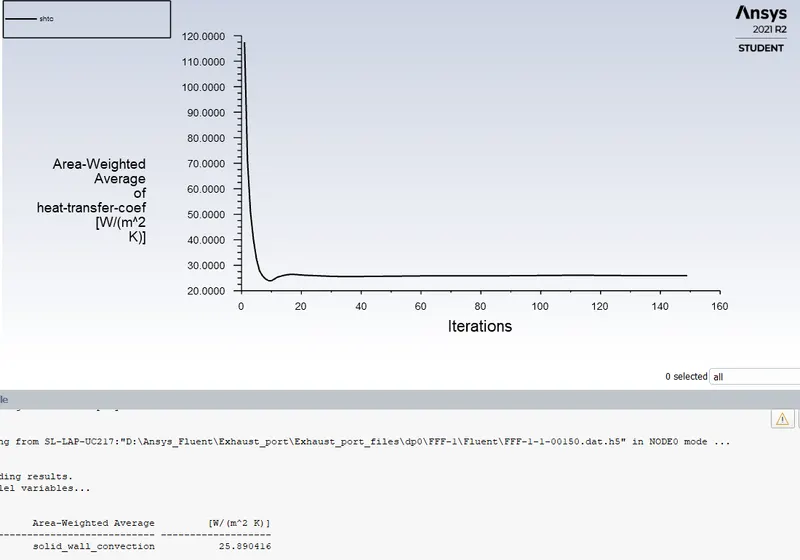Case 3 k-Omega

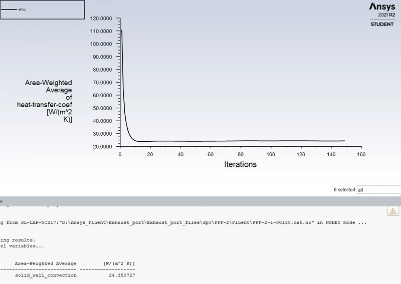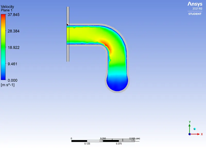
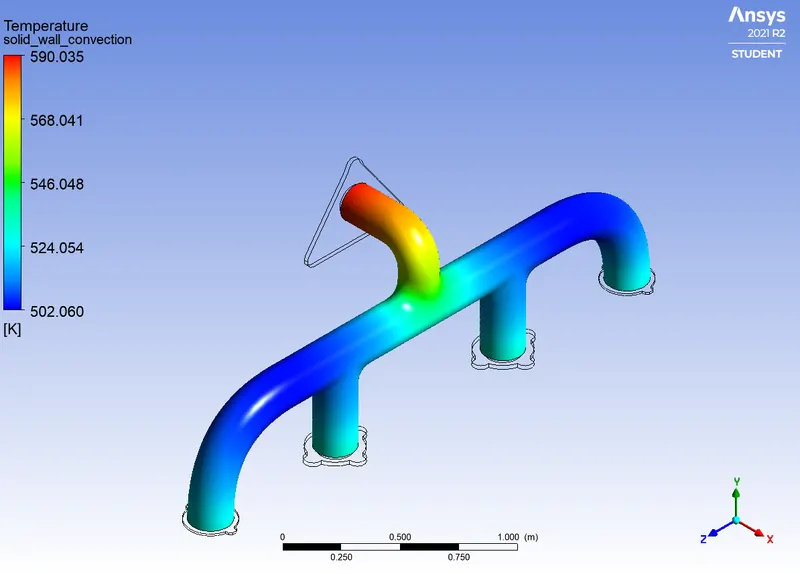
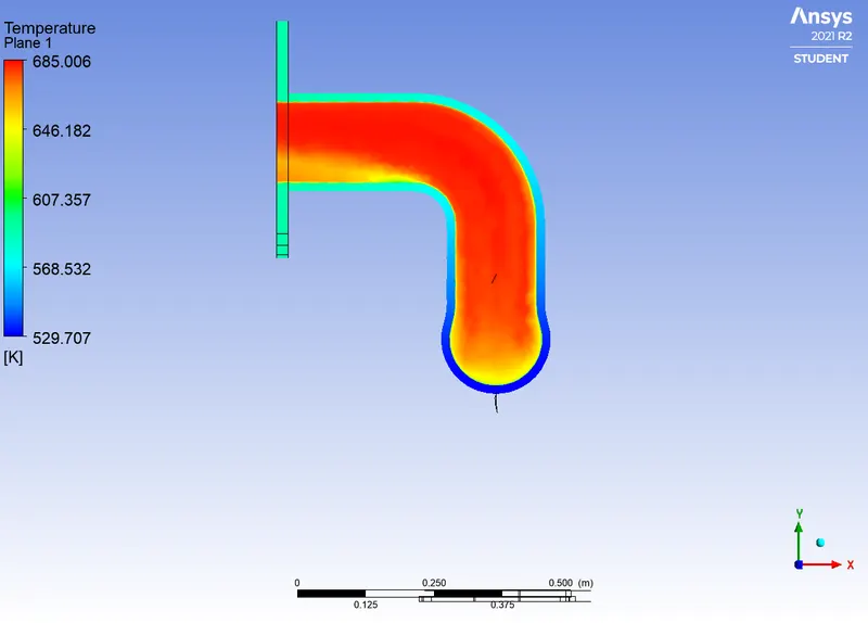
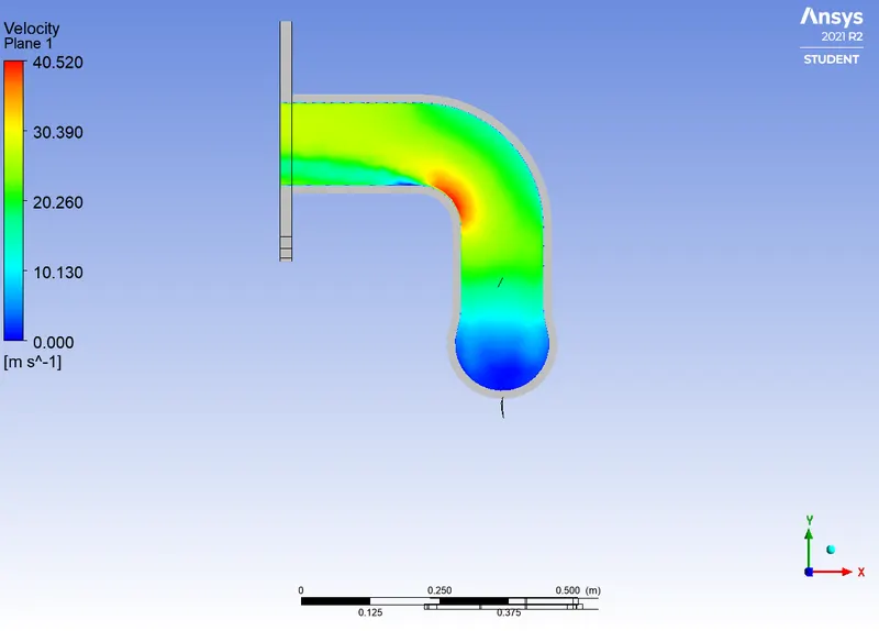
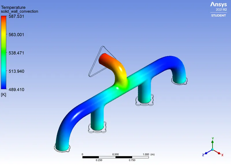
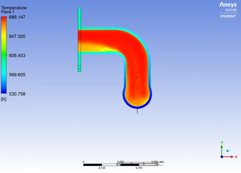
The results obtained after conducting the simulations are shown in the form of contours shown below:

Case 1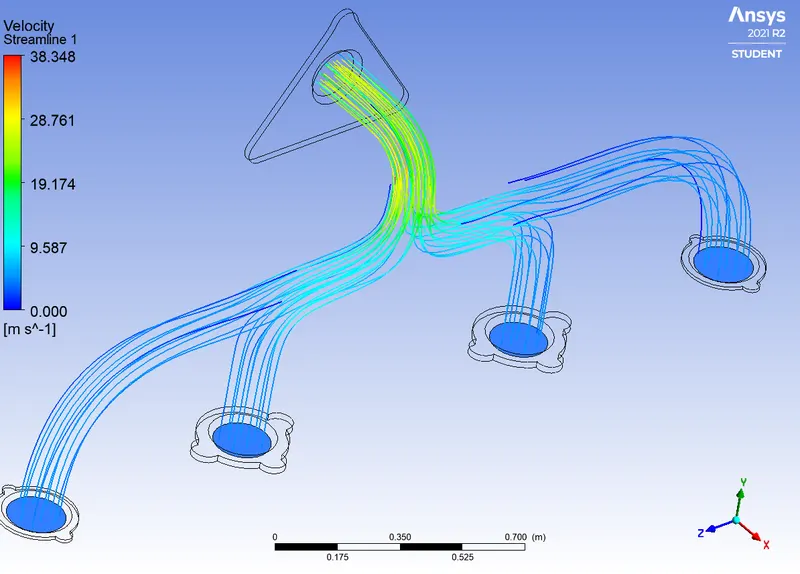

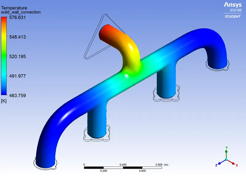Case 2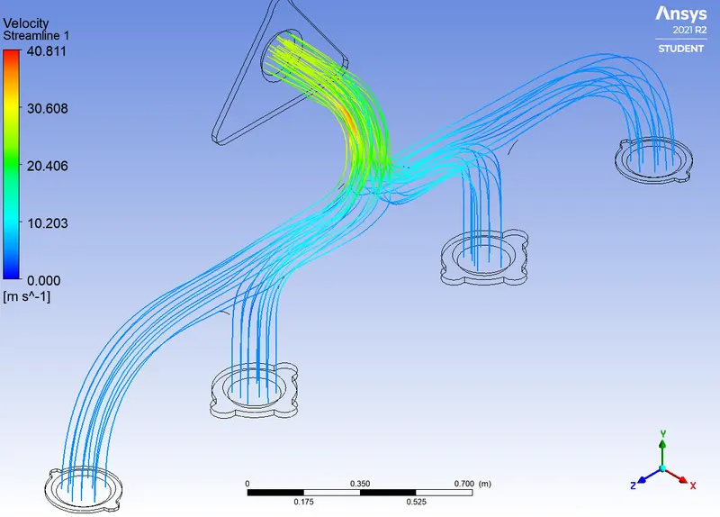

Case 3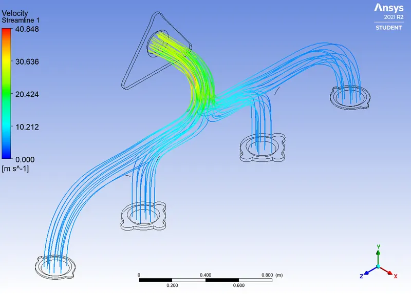

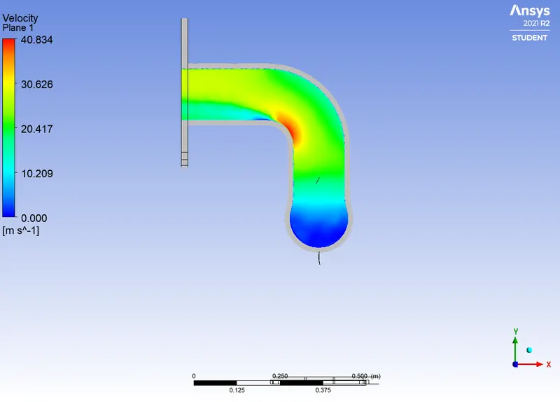The above results clearly show the difference between the various cases employed. Due to the Difference between the grids in case 1 and case2, case3 the resoultion captured withh the surfacce heat tranfer coeff is different. Though, for the case 2 and 3 there is clear difference between the HTC. Although the when  it comes to the which model performed better analytical validation is needed for the comparision. 

For analytical validation, there exist a realtion between the Nusslet number, Reynolds number and Prandlt number. 

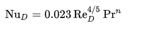
This relationship is established with experiments for the trubulent flow in pipes.

In conclusion it has been observed with comparitive study that the models used and their accuracy will be based on the analyical validation. Moreover, as observed from the plots the velocity increaes at the throat region which gives rise to the HTC at that area as the mass flow rate also increases. This is quite important as it would help in optmizing the design of the exhaust port.