Week 5 - Rayleigh Taylor Instability
Reyleigh Taylor instability: A phenomenon observed in the naure is wen 2 fluids wih different velocities are moving with different velocites and an interaction takes place between them wich is an initiation of mixing. The pattern created by this is important indicaation of the mixinig ability of both fluids. This period of begining of the mixing is known as Reyleigh Taylor's instability.
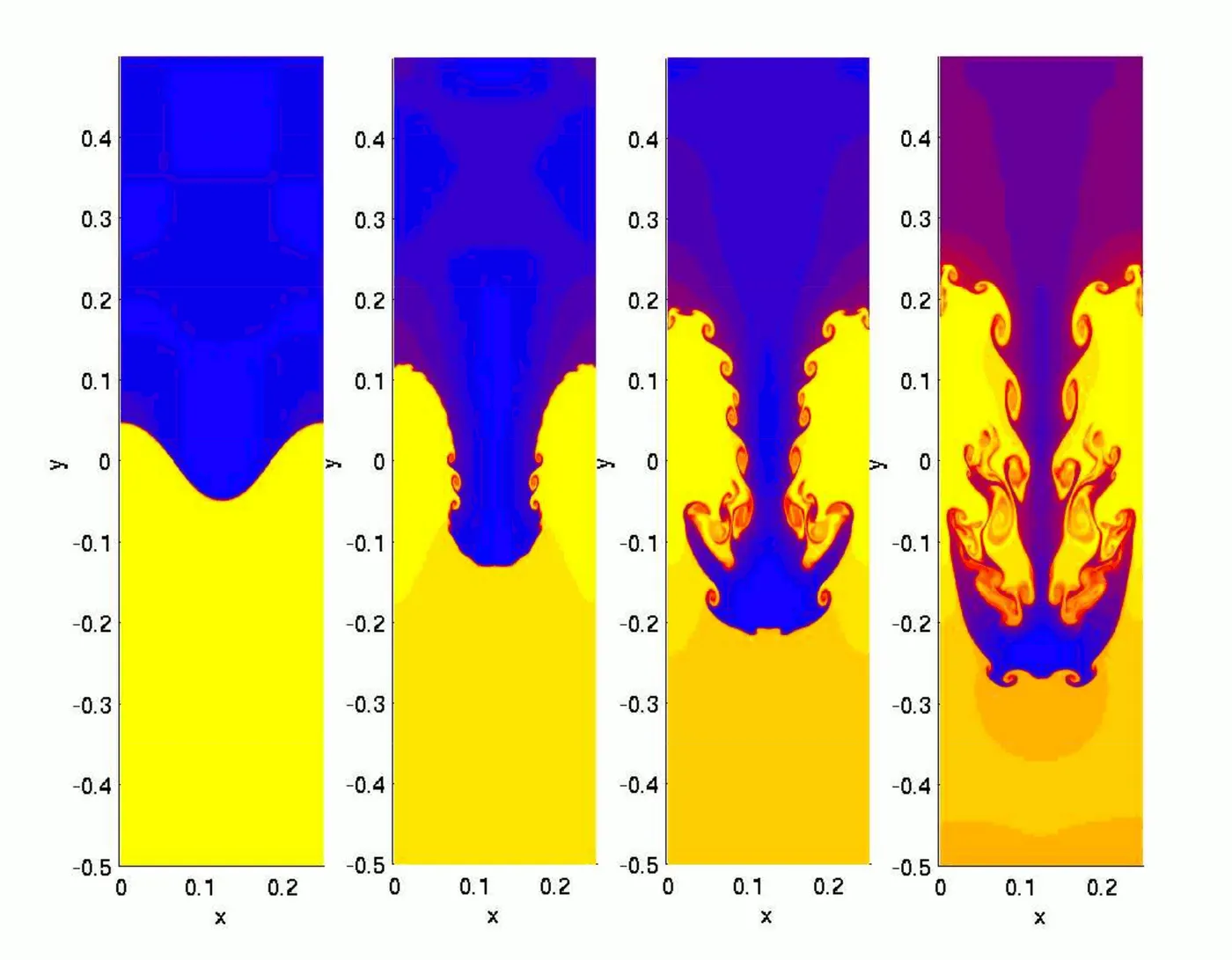 |
The above image shows 2 fluids of different velocities thata are mixing. As we can see a few instabilities occuring in the begining and then as the denser fluid is on top of the less dense fluid due to the efefct of the gravity we can observe "finger" in the second image.
Atwood number: The Atwood number is signifies the hydraulic instabilities in densities of fluids, it is a dimentionless number.
Given by,
`A = (rho1-rho2)/(rho1+rho2)`
THere are a few mathematical models used to study the Reyleigh Taylor instability such as:
1) Kelvin-Helmholtz instability: This ccurs when there is a relative motion between 2 fluids of different densities over one another. Due to this swirling shapes occure that then proceed to mixing.
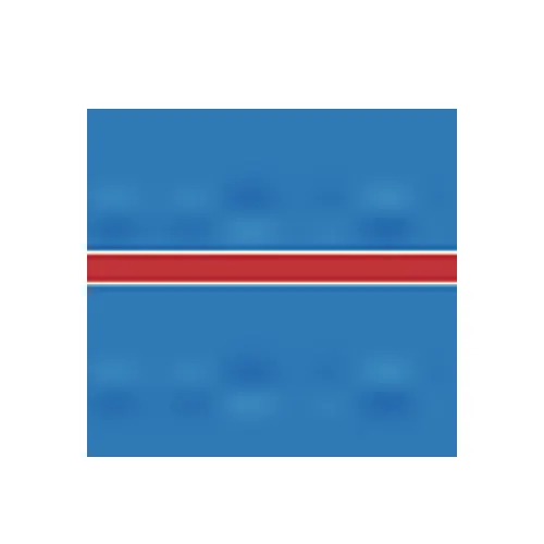 |
mathematically this is expressed as:
2) Saffma-Taylor instbility: This is inverse Reyleigh-Taylor instability, where a less viscous fluid is injected into the fluid with higher viscosity. the high viscosity fluid leaves finger like structure. There exist other types of instabilities as well whic are slight variations of Reyleigh-Taylor instablity.
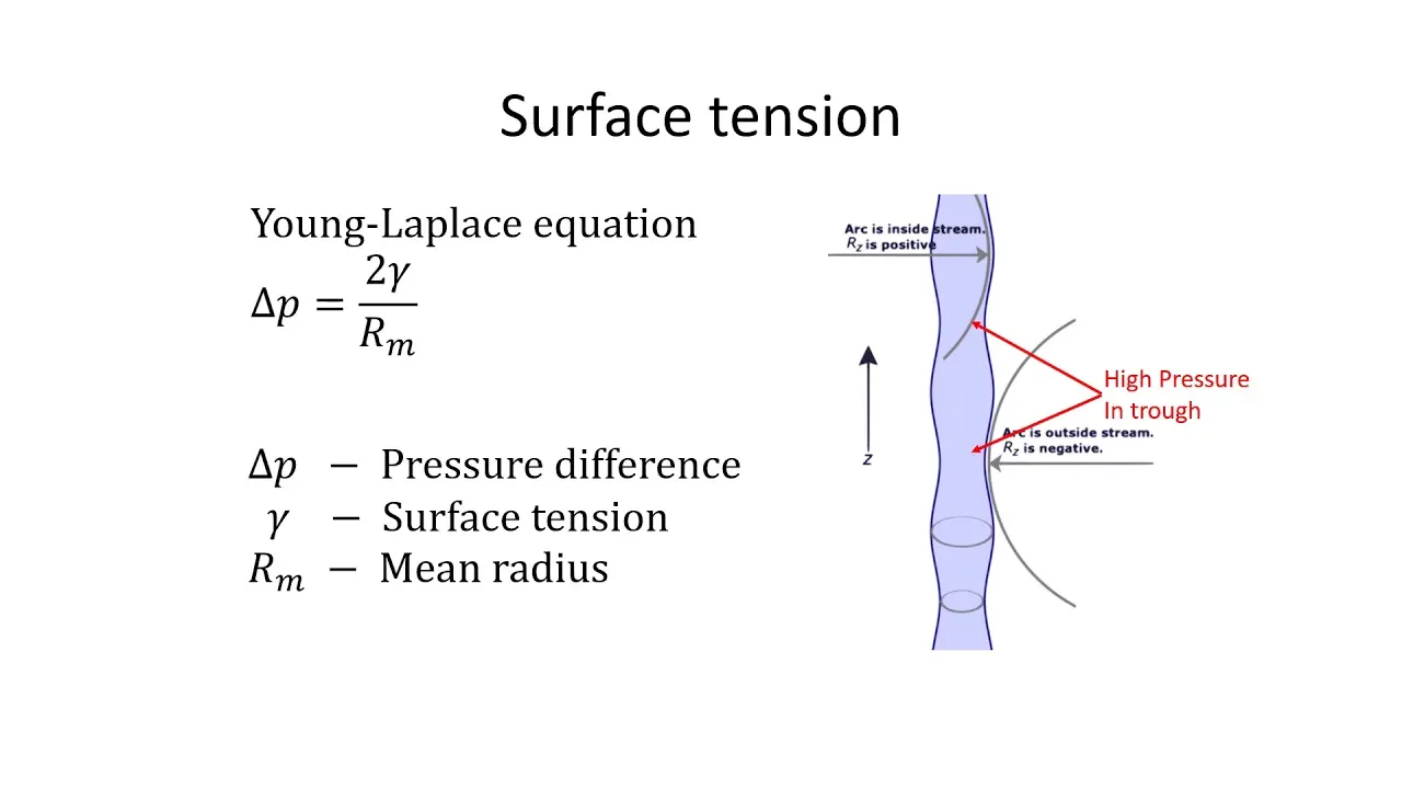
3) Plateau-Rayleigh instability: It explains why and how a falling strea, of fluid breaks up into smaller packets with the same volume but less surface area.
 |
Why Steady state is inappropriate?
Steady state simulation are equipped to solve Navier-Stokes equations but as they are concerned with reaching to the steady state only and we do not get to see how the flow will unfold in time, which is crucial in this case as the assessment of occurence of instabilities is important and it is seen with Transient simulation only.
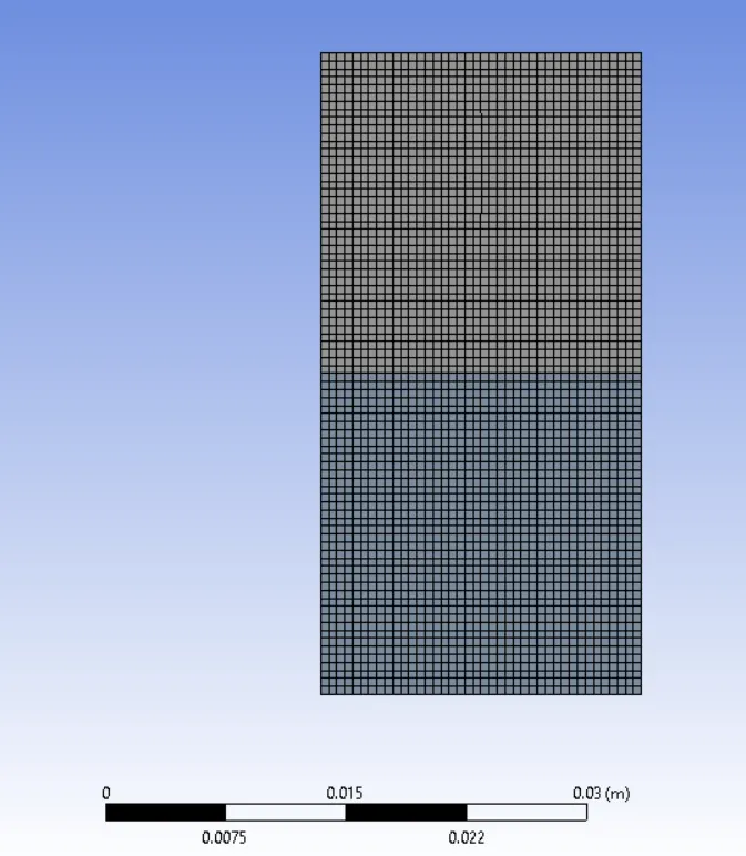
The simulation conducted was for 2 cases of grid size 0.5mm.
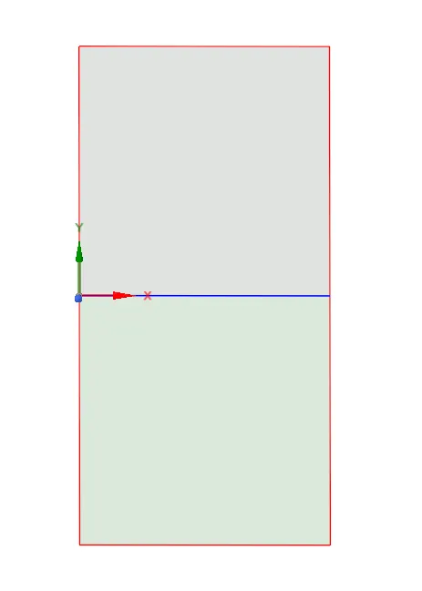
The geometry is created in space claim and share topology is enabled fluid (Air and Water) domain.
 |
further mesh created is as below:
 |
Case setup:
A laminar model is used for the simulation with multiphase enables (air and water) for one case and custom fluid with air for another.
Post initialization patching is done to assign the fluid to the respective region.
For 2 cases the denser fluid water and a custom material (density = 400 kg/m3, viscosity = 0.001 kg/m-s) were assumed:
A laminar solver is used with mutiphase is turned on. Phases selection is done post initialization.
Results:
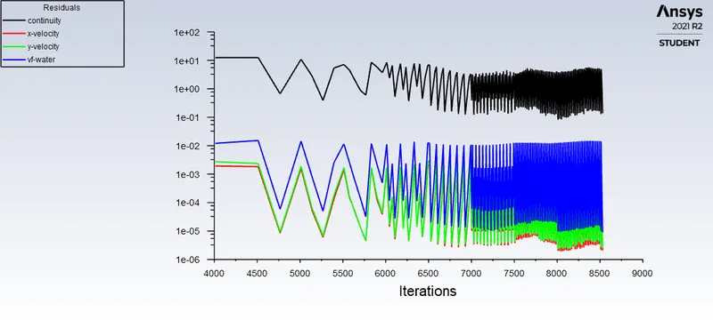
Case 1 : Water
 |
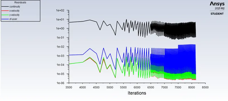
Case 2: Userdefined fluid.
 |
The animation result has been attached as follows:
| Case 1 with water | Case 2 User |
The atwood number for each case is given by:
A(Case 1) : 0.9975
A(Case 2) : 0.4
Conclusion: Instabilities can occure in nature as well as industrial systems, being able to understand how they occre we can understand the implications of them. CFD gives a good understanding of these phenomenons.