Week 1- Mixing Tee

Introduction:

The following simulation is done in order to understand the mixing efficiency of fluid (air) a different temperatures. i.e Hot (`36^oC`) and Cold (`19^oC`). Also, to have an understanding of RANS models

k-Epsilon-Realizable and k-Omega SST.

The problem is broken into different cases as per the requirement.

Case 1	Short T-joint with momentum ratio of 2	To understand the effects of each viscous model
Case 2	Short T-joint with mmentum ratio of 4
Case 3	Long T-joint with Momentum ratio of 2
Case 4	Long T-jont with Momentum Ratio of 4	This case was used to undertake Grid independence study.

The results and inferences are discussed below:

Case 1:

Short T-Joint with Momentum ratio of 2:

Based on the metioned specifications the simulation was conducted.

Mesh element size : 5e-3 with 14062 elements.

Hot inlet: 3 m/s at `36^oC`

Cold inlet: 6 m/s at `19^oC`

k-Epsilon	k-Omega

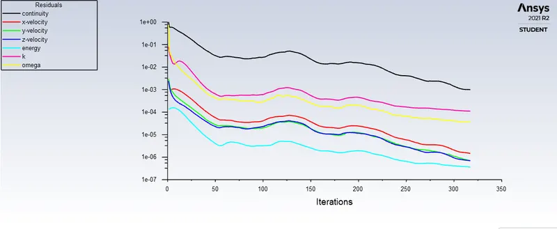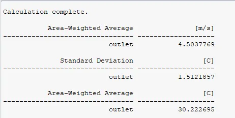
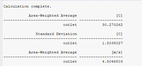
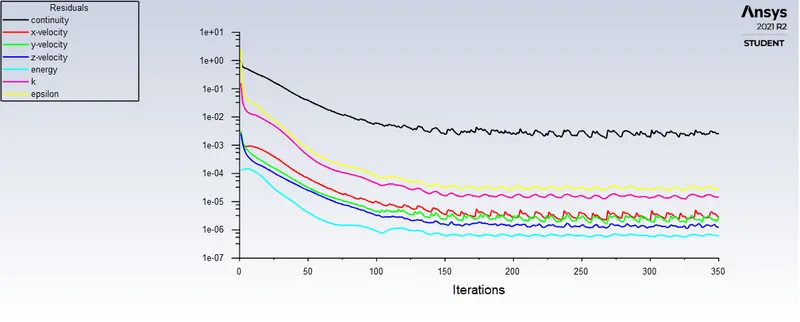
From above table it seems clear that the values obtained for average temperature and SD of the temperature is same. But the solution converged for k-Omega at 317th iteration whereas the for the k-epsilon oscillations were seen. As the oscillations are not repetative nor the solution converge for the k-epsillon model for further study k-omega was used.

Results:

Post-Processing:

Temperature along the length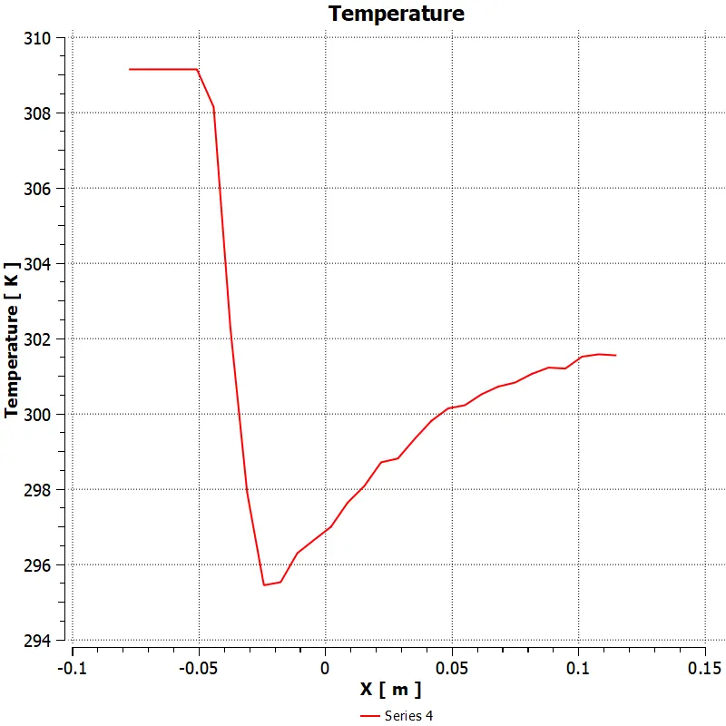
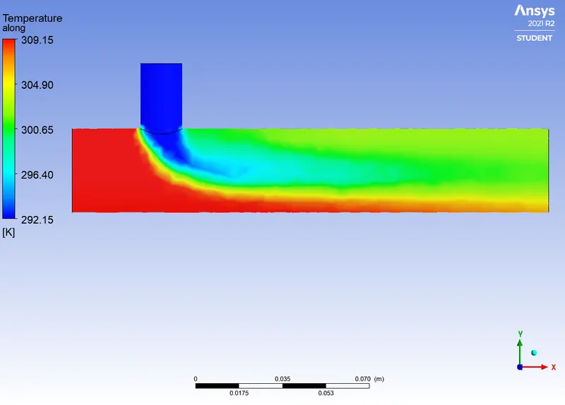Temperature across the width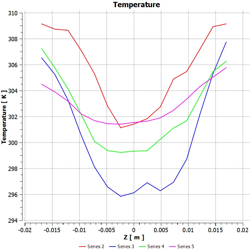

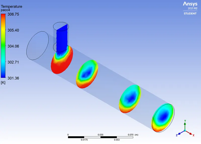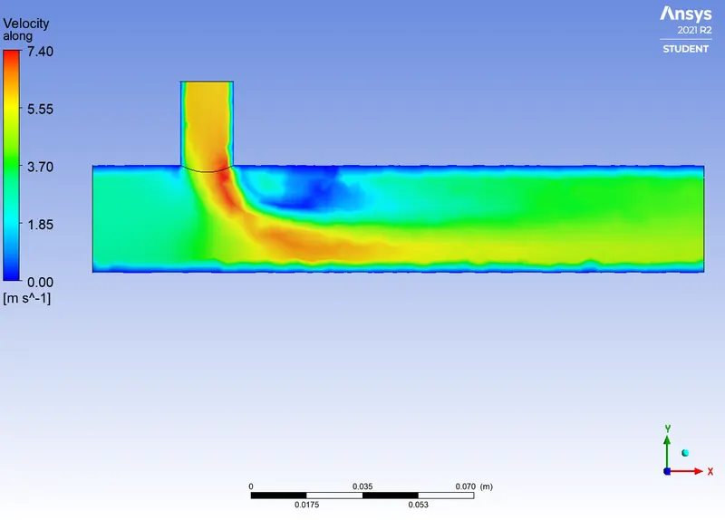
Velocity along the length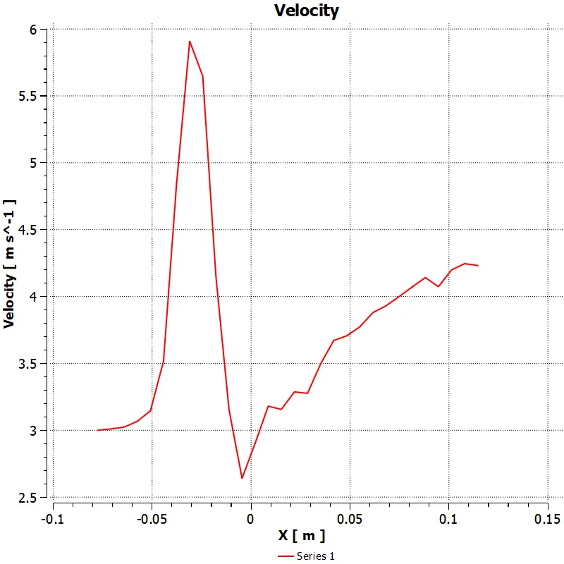
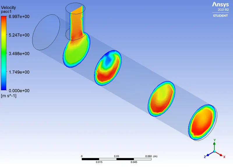
Velocity across the width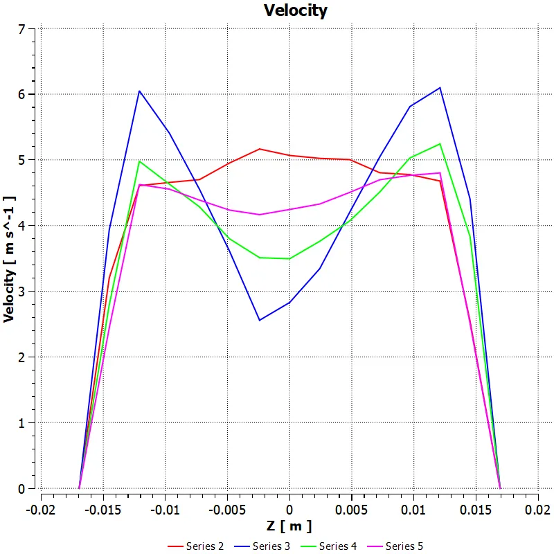

Case 2:

Short T-Joint with Momentum ratio of 4

The mesh configuration is same as the previous case.

Hot inlet: 3 m/s at `36^oC`

Cold inlet: 12 m/s at `19^oC`

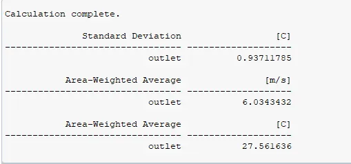
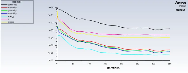
Result	Residual

Post-Processing:

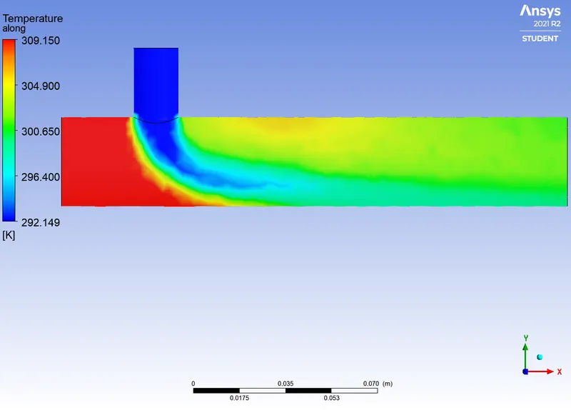
Temperature along the length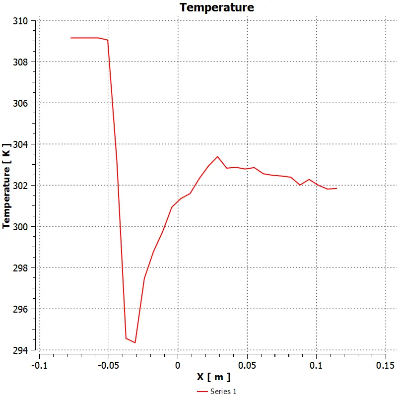
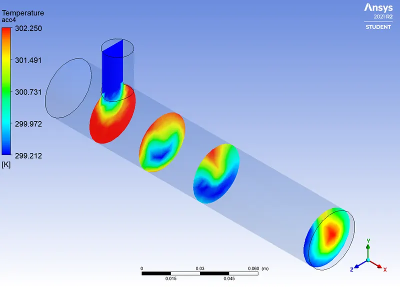
Temperature across the width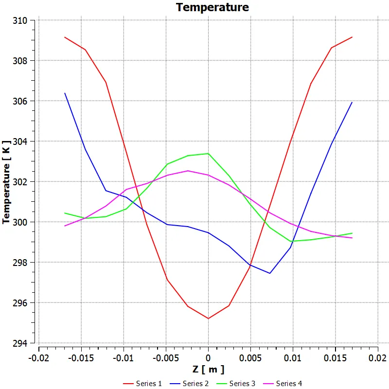

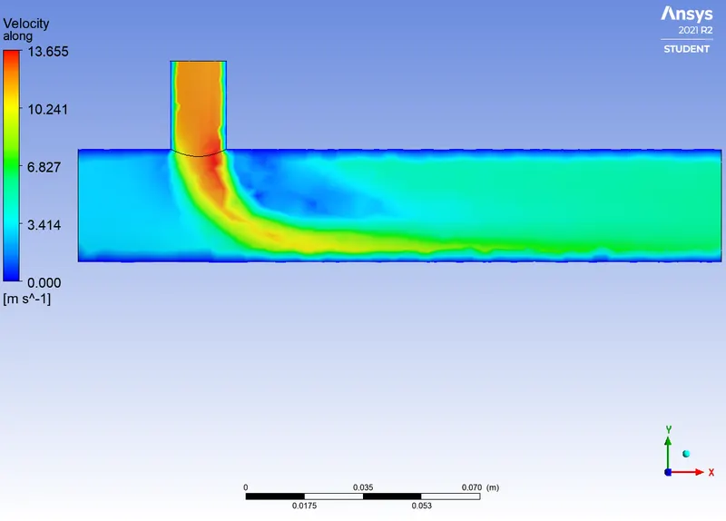
Velocity along the length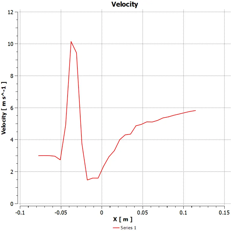
Velocity across the width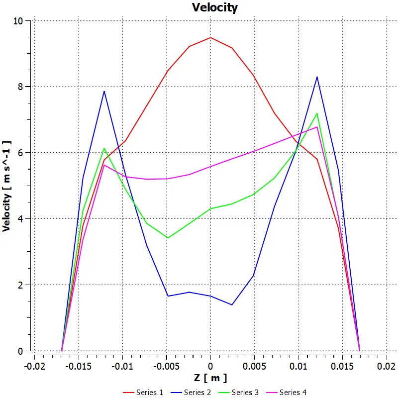

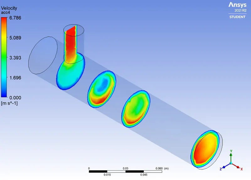Case 3:

long T-joint with momentum ratio of 2

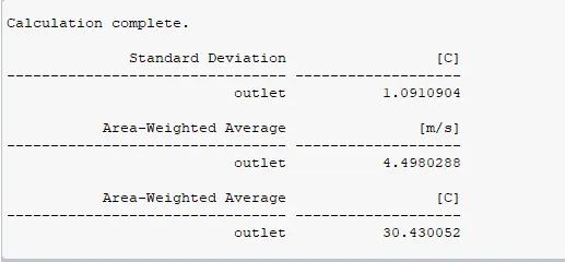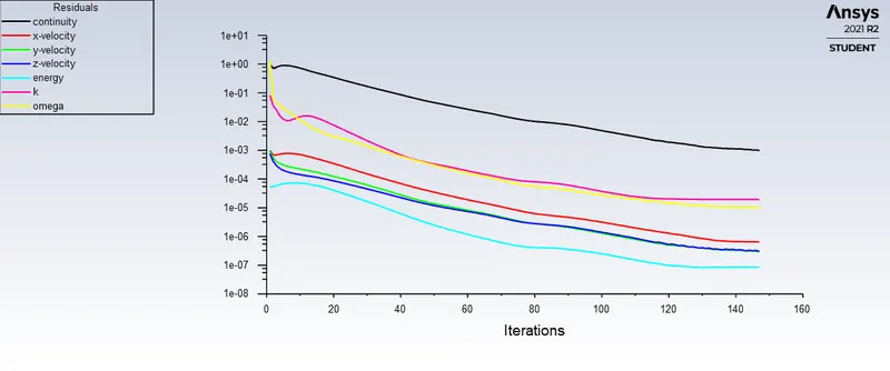Post-Processing:

Temperature along the length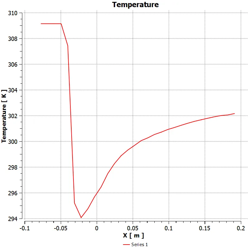
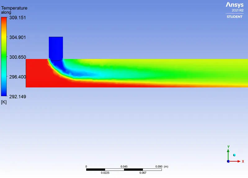Temperature across the width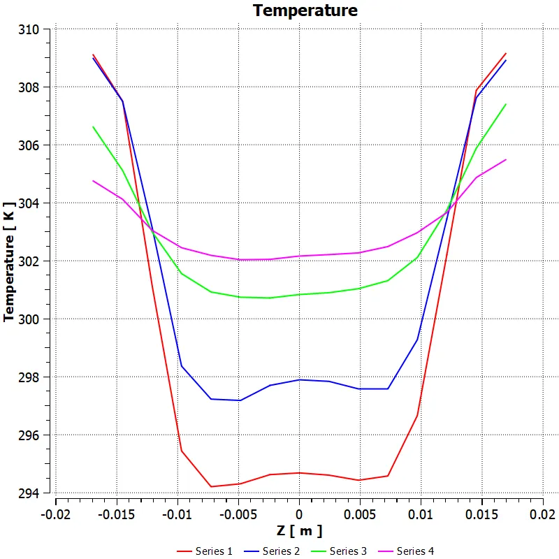

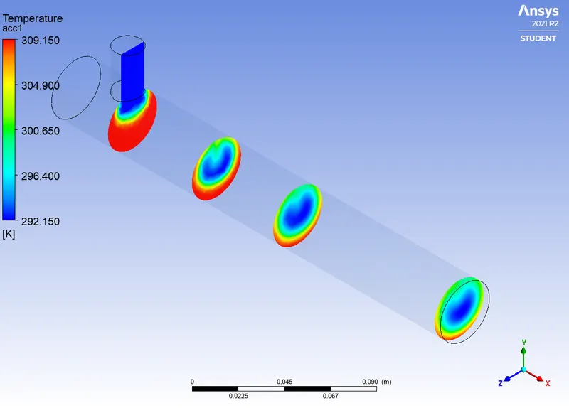Velocity along the length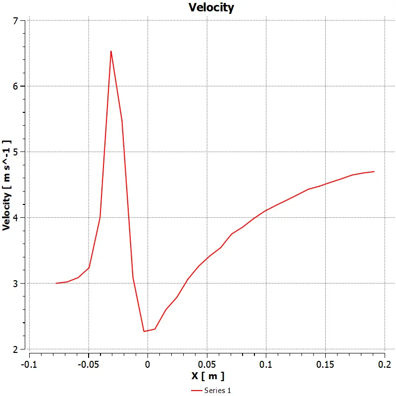
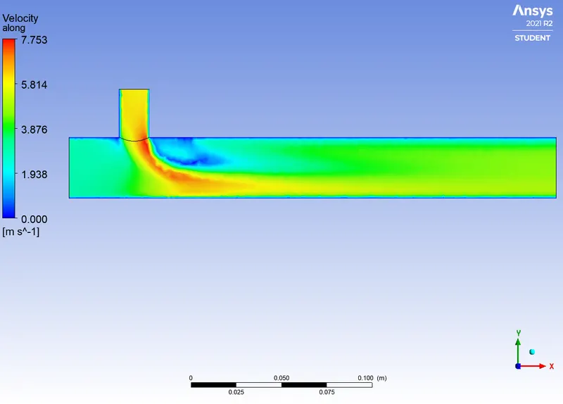Velocity across the width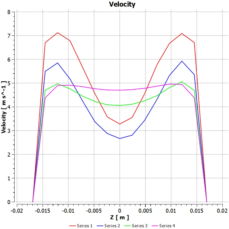

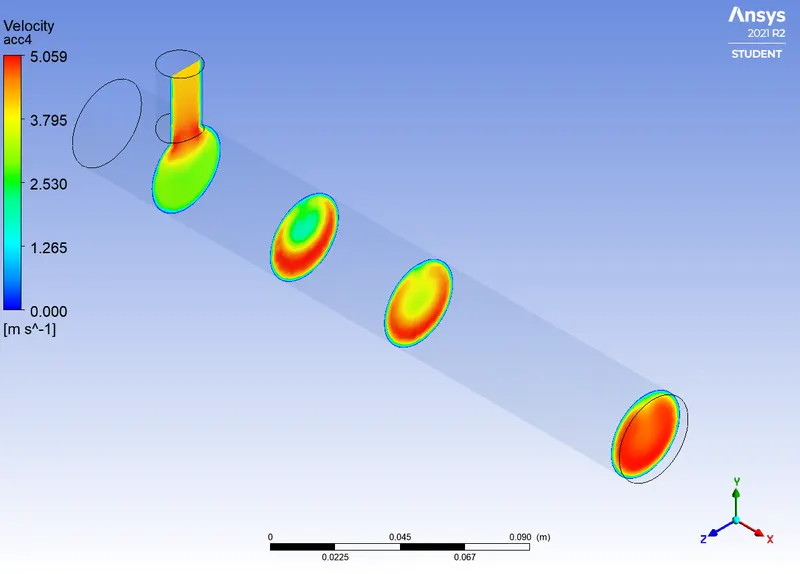Case 4:

long T-Joint with momentum ratio of 4

This case was considered for the grid convergence test.

the table below shows the result of the test.

Grid1	Gid2	Grid3
Default 15566	7e-3: 28648	2e-3: 138800
	Converged at 174	Convergerd at 241

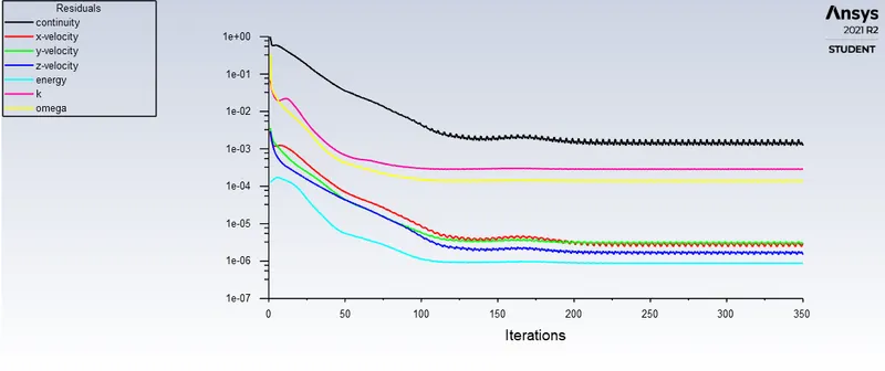
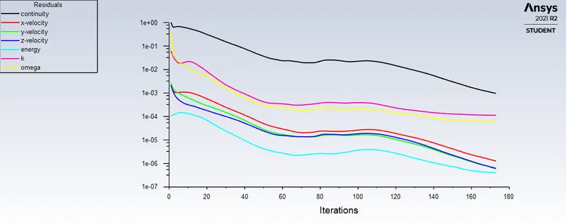
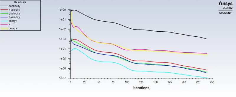
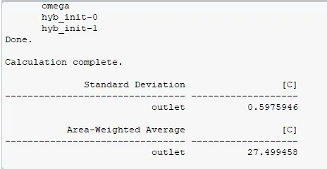
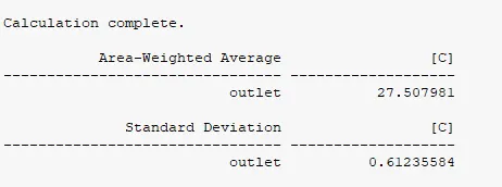
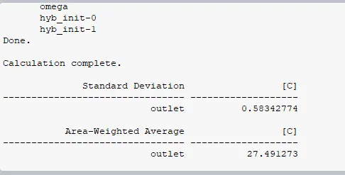
From the above values it is evident that there seems to be very less deviation from the default value. This goes for both the Standard deviation and Average temperature. With this we can conclude that the default mesh is is equally accurate as the more refined mesh. Although, by no means it can e concluded that the obtained outlet temperature is accurate as it need to be comare with the analytical value.

Post-Processing:

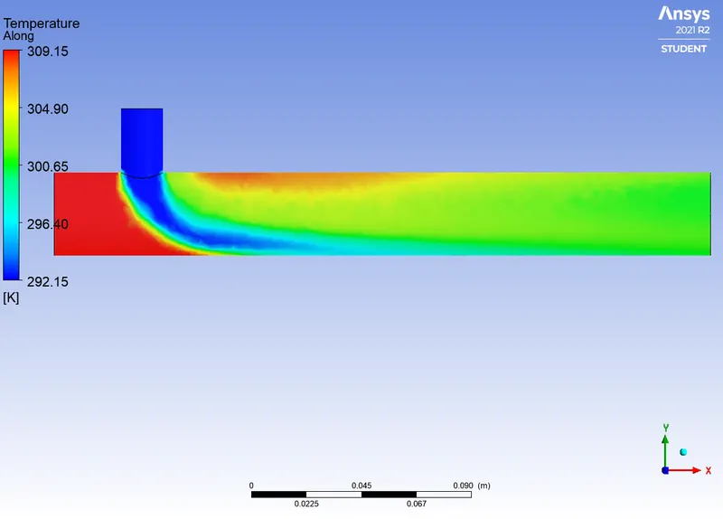
Temperature along the length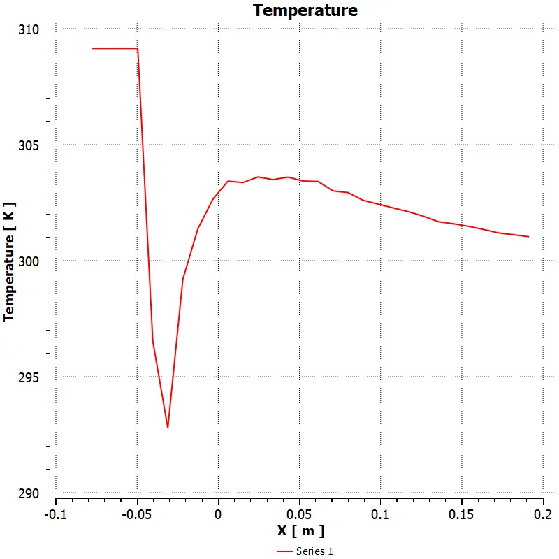
Temperature across the width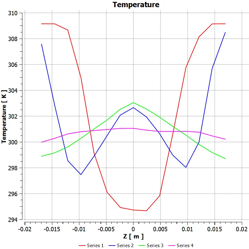
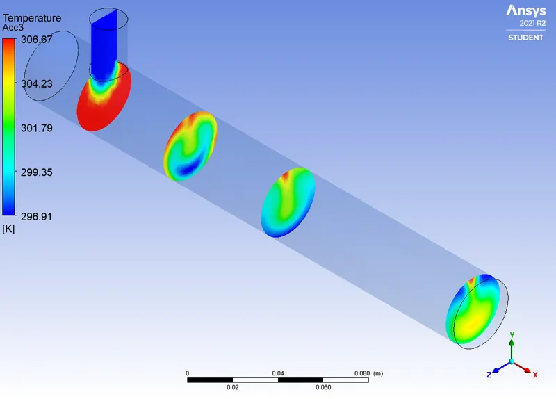Velocity along the length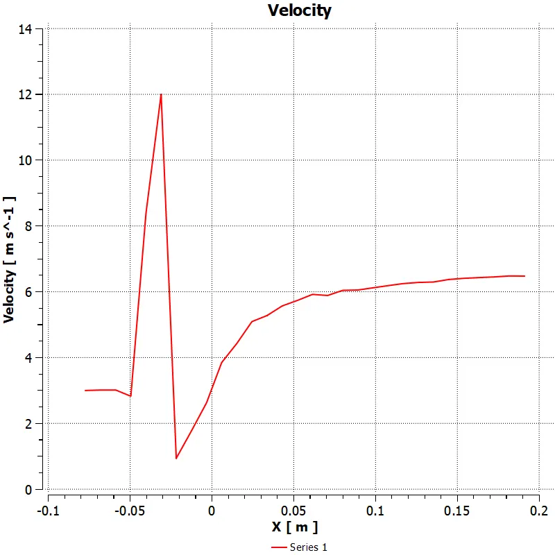
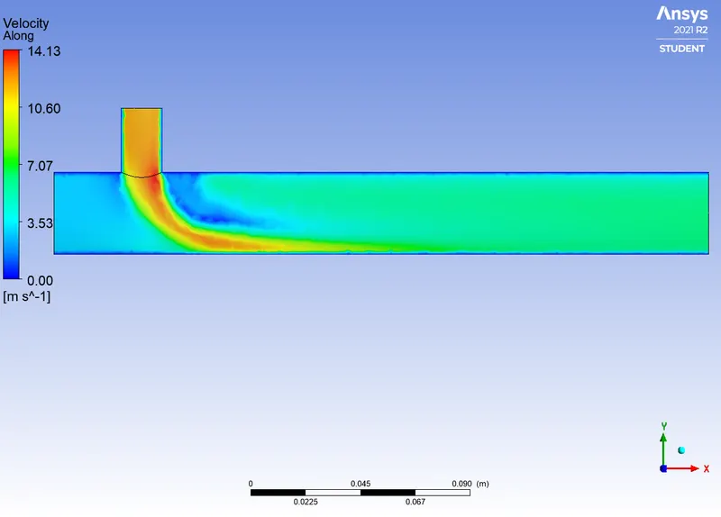Velocity across the width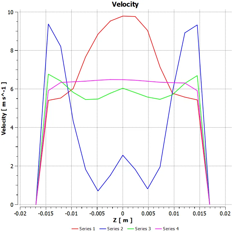

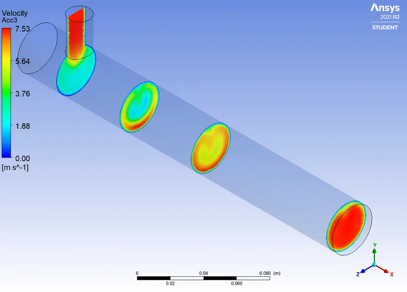Conclusion:

In conclusion based on the residual and the fact that the k-omega (sst) model converged it was choosen to conduct further studies. Also, the k-omega model is more robust as it is a combination of the k-epsilon and k-omega. Eventhough the k-epsilon model is good at any given boundary conditions it falters sometimes and was not suitable for this study. Furthermore, for the grid independence the default mesh gave the same result as the most refined mesh, this means that the the default mesh is good enough to have accurate result. Also, mesh refinement near wall could have give better results near the wall.