Week 5 - Rayleigh Taylor Instability

RAYLEIGH TAYLOR INSTABILITY:-

Aim.

To Perform the CFD simulation of Rayleigh Taylor Instability with different mesh sizes and user-defined material.

Objective.

1. what are some practical CFD models that have been based on the mathematical analysis of Rayleigh Taylor Waves? In your own words, explain these mathematical models that have been adapted for CFD calculation.
2. Perform the Rayleigh Taylor instability simulation for 2 different mesh sizes with the base mesh being 0.5 mm. Compare the results by showing the animations (Attach them from google drive). Observe the differences in the animation and explain the effect of mesh size on simulation. Also, explain why a steady-state approach might not be suitable for this type of simulation.[choose Air and water for this simulation]
3. Run one more simulation with water and user-defined material(density= 400 kg/ `m^3`, viscosity =0.001 kg/m-s) for refined mesh.
4. Define the Atwood Number. Find out the Atwood number for both the cases and explain how the variation in Atwood number in the above two cases affects the behavior of the instability.

Introduction & Theory.

1. Rayleigh-Taylor Instability:-

• The Rayleigh-Taylor instability is the instability of an interface between two fluids of different densities which occurs when the lighter fluid is pushing the heavier fluid. Examples include the behavior of water suspended above oil in the gravity of Earth, mushroom clouds like those from a volcanic eruption and atmospheric nuclear explosions, supernova explosions in which expanding core gas is accelerated into denser shell gas, instabilities in plasma fusion reactors, and inertial confinement fusion.
• Water suspended atop oil is an everyday example of Rayleigh - Taylor instability, and it may be modeled by two complete plane=parallel layers of immiscible fluid, the denser on top of the less dense one and both subject to the earth's gravity.
• The Equilibrium here is unstable to any perturbation or disturbance of the interface: if a parcel of heavier fluid is displaced downward with an equal volume of lighter fluid displaced upwards, the potential energy of the configuration is lower than the initial state. Thus the disturbance will grow and lead to a further release of potential energy, as the more dense material moves down under the gravitational field, and the less dense material is further displaced upwards. This was the set-up as studied by Lord Rayleigh.
• The difference in the fluid densities divided by their sum is defined as the Atwood number.

CFD models that have been based on the mathematical analysis of Rayleigh Taylor Waves:

• Plateau - Rayleigh instability
• Kelvin - Helmholtz instability
• Richtmyer - Meshkov instability
• Saffman - Taylor instability

A. Plateau - Rayleigh instability.

• The Plateau - Rayleigh instability is a falling stream of fluid that breaks up into smaller particles with the same volume but less surface area. This fluid instability is exploited in the design of a particular type of inkjet technology whereby a jet of liquid is perturbed into a steady stream of droplets.

B.Kelvin -Helmholtz instability.

• The kelvin - Helmholtz instability typically occurs when there is velocity shear in a single continuous fluid or velocity difference across the interface between two fluids. A common example is seen when the wind blows across a water surface, the instability constant manifests as waves.
• Kelvin - Helmholtz instabilities are also visible in the atmosphere of planets and moons, such as in cloud formation on earth or the red spot on Jupiter and the atmospheres of stars, including the sun.

C. Richmyer - Meshkov instability.

The Richmyer - Meshkov instability occurs when two fluids of different densities are impulsively accelerated. Normally this is by the passenger of a shock wave. The development of the instability begins with small amplitude perturbation which initially grows linear with time.

This is followed by a nonlinear regime with bubbles appearing in the case of a light fluid penetrating a heavy fluid, and with spikes appearing in the case of a heavy fluid penetrating a lighter fluid. This instability can be considered the impulsive-acceleration limit of the Rayleigh - Taylor instability.

D. Saffman - Taylor instability

The Saffman - Taylor instability, also known as viscous fingering, is the formation of patterns in a morphologically unstable interface between two fluids in a porous medium. Most experimental research on viscous fingering has been performed on Hele-Shaw cells, which consist of two closely spaced, parallel sheets of glass containing a viscous fluid.

2. Define Atwood Number.

The Atwood number (A) is a dimensionless number in fluid dynamics used in the study of hydrodynamics instabilities in density stratified flows. It is a dimensionless density ratio defined as

`A = (rho_1 - rho_2)/(rho_1 + rho_2)`

where,

`rho_1` = density of the heavier fluid

`rho_2` = density of the lighter fluid

Application:-

Atwood number is an important parameter in the study of Rayleigh - Taylor instability and Richmyer - Meshkov instability. In RT instability, the penetration distance of heavy fluid bubbles into the lighter fluid is a function of the acceleration time scale.

SIMULATION PROCESS:-

In the Rayleigh Taylor Instability, the three sets of cases have been simulated.

• Case 1 - Baseline Mesh of 0.5mm Element size.
• Case 2 - Refine Mesh of 0.2mm Element size.
• Case 3 - Refined Mesh with User-defined material.

CASE - 1:-

1. Geometry (Spaceclaim).

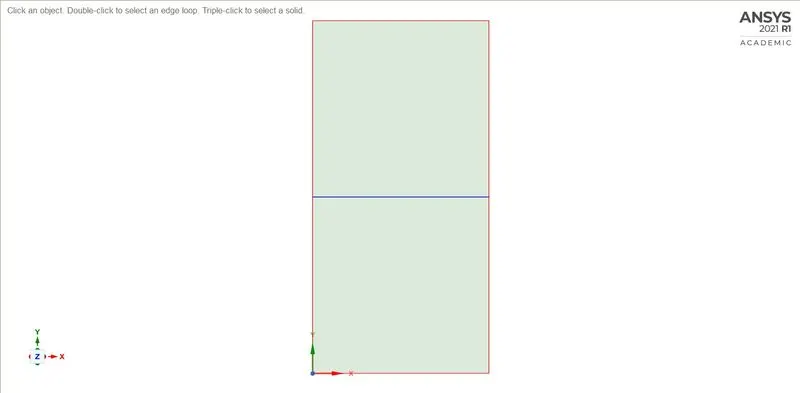
• In SpaceClaim, the two geometry (Air and Water) has been created by 20 X 20 mm.
• The air is in the bottom region and water is in the upper region.
• And Pull the geometry as a surface.
• Share the topology between the two-fluid.

Sketch Preparation (Air & water):-

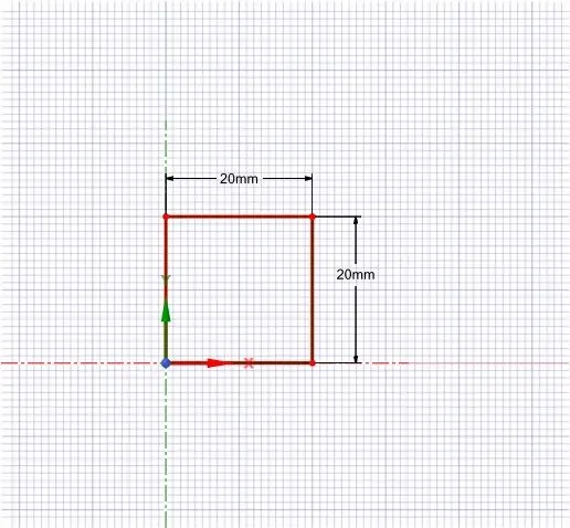
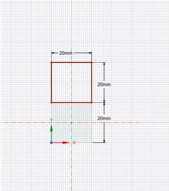
(a). Air (b). Water

Geometry (Air & water):-

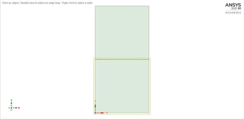
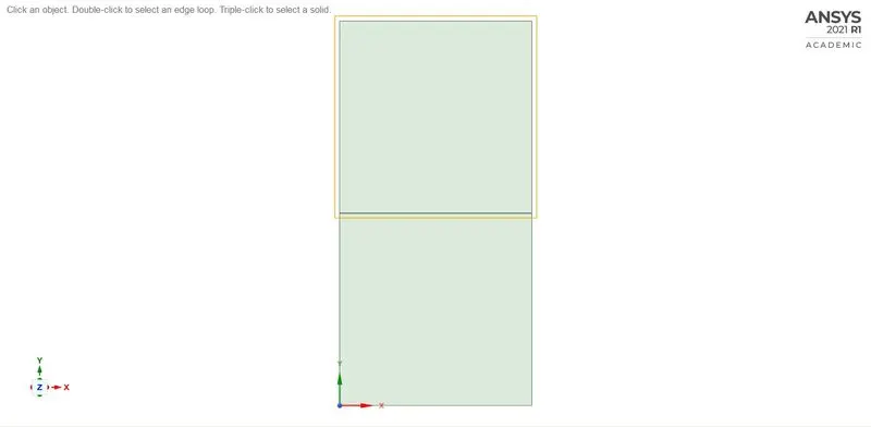
(a). Air Region (b). Water Region

Share Topology:-

2. Meshing.

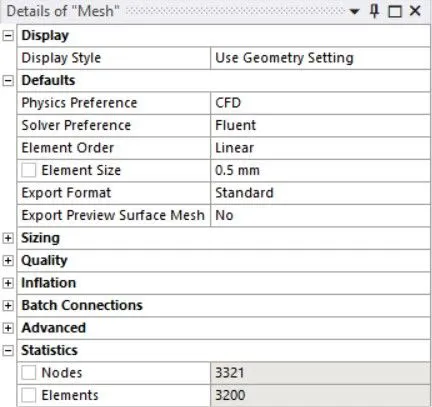
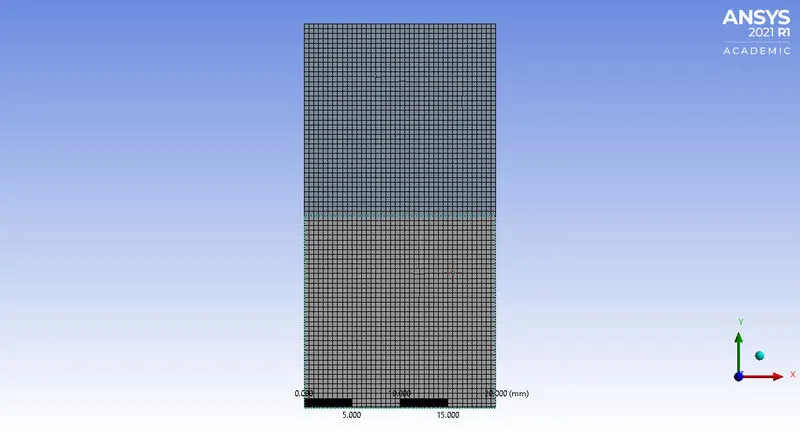
• Meshing the geometry with a baseline of 0.5 mm.
• Elements = 3200

3. Setup and Solving (Fluent).

A. Solver

• The transient-state calculation is performed.
• A pressure-based solver and Absolute velocity are used.
• Gravity is enabled in -ve Y-axis (9.81`m//s^2`)

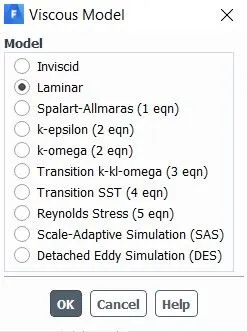
B. Viscous model = Laminar

C. Multiphase Model.

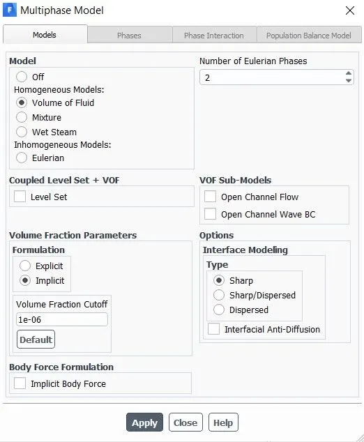
Multiphase Model is turned on along with Volume of Fluid and number of Eulerian phases is chosen as 2 and implicit formulation is selected.

D. Material.

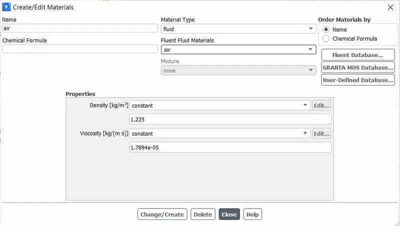
• Air

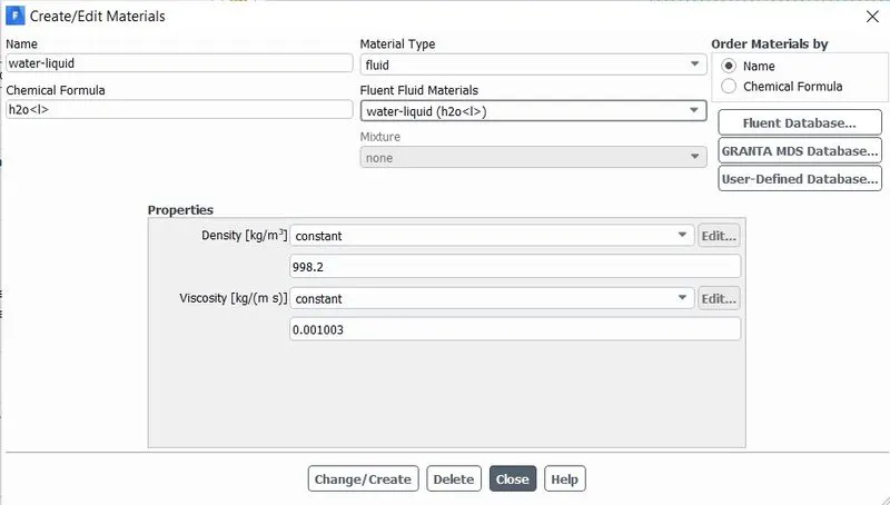
• Water

E. Phases.

• Air is the Primary phase.

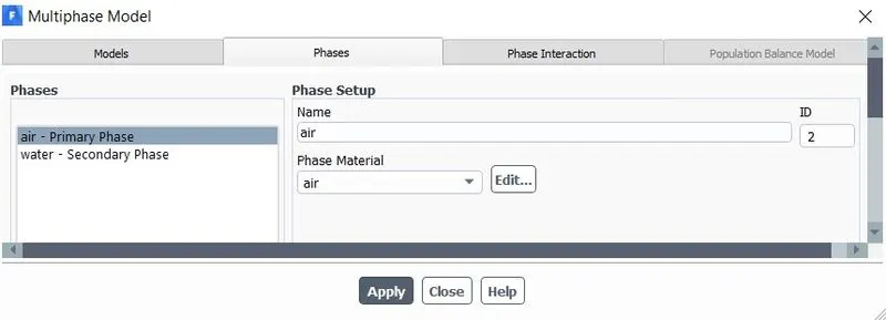
• Water is the Secondary phase.

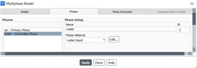
F. Initialize with the Standard method.

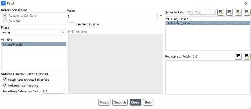
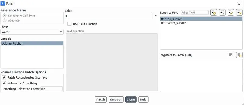
G. Patch.

• Patching of the volume of the two phases is performed before the start of the simulation. The phase used for patching was water and a volume fraction of 1 is taken for water surface and 0 for air surface.

H. Contour.

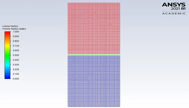
From the contour the patches are correct. Run the simulation for

• Time step = 0.005
• No. of time step = 1500

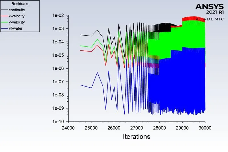
Residuals:-

4. Post-Processing Result.

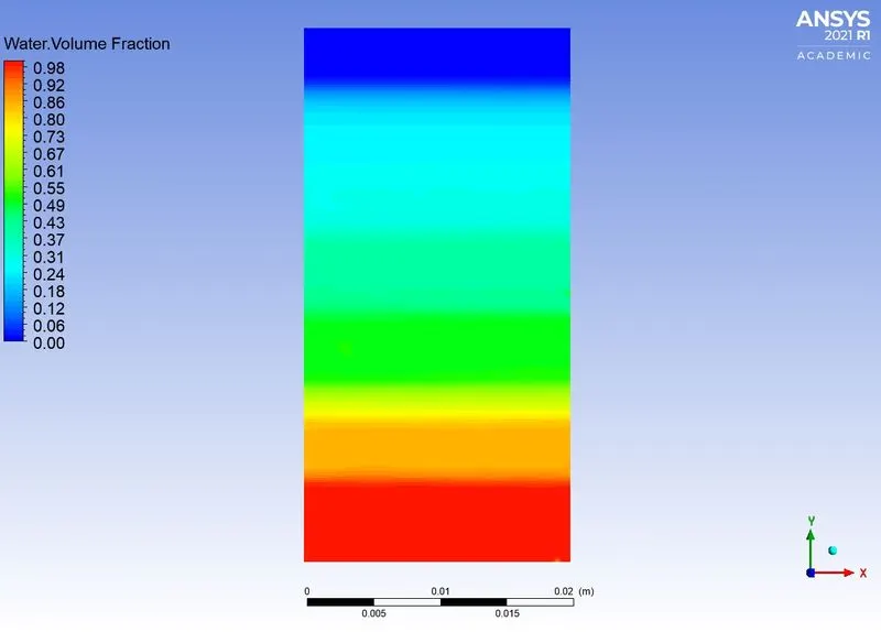
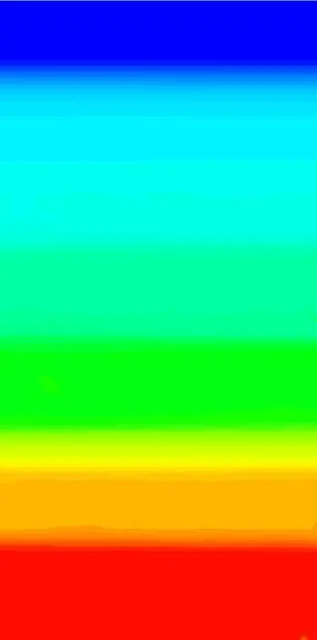
1. Water Volume Fraction contour:-

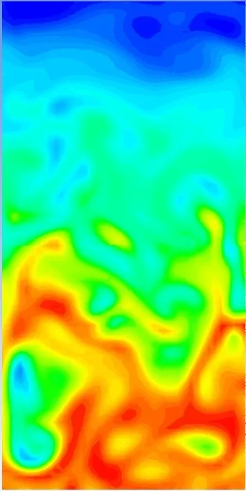
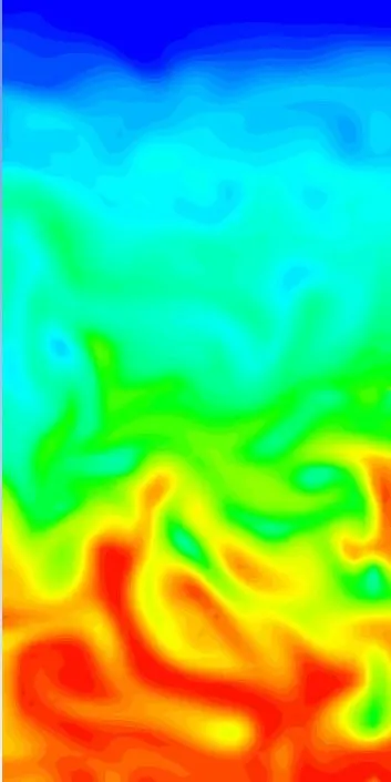
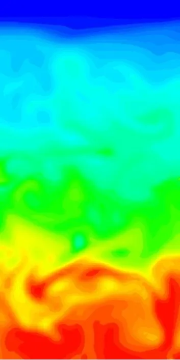
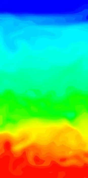
2. Penetration of heavier fluid into the lighter fluid at different Time steps.

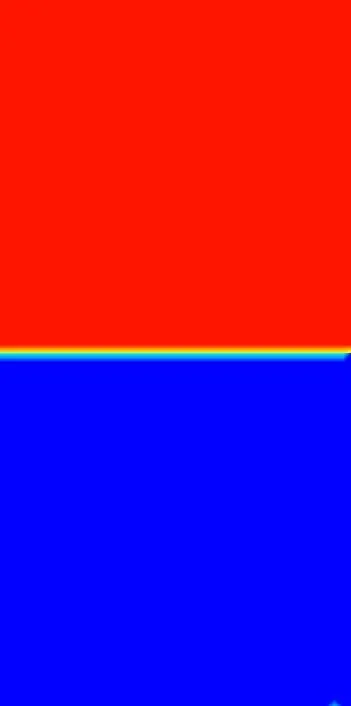
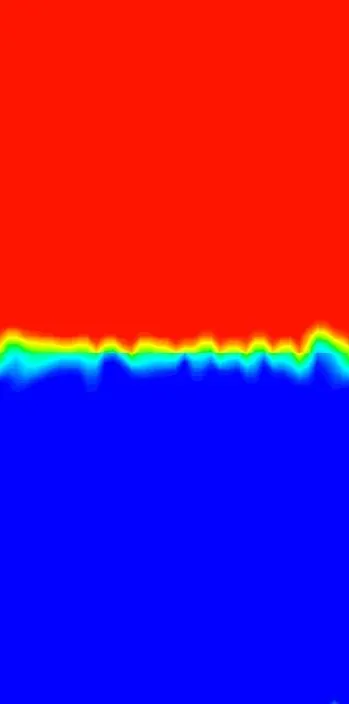
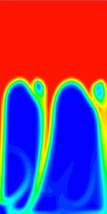
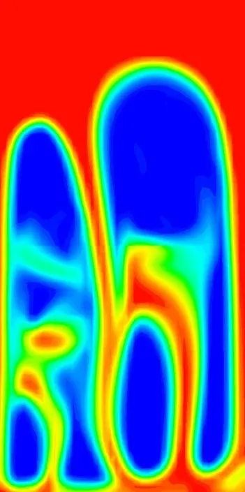
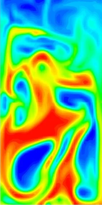
(a) 0.025s (b) 0.075s (c) 0.15s (d) 0.25s (e) 0.5s

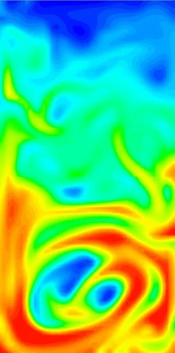
(f) 0.75s (g) 1s (h) 1.25s (i) 1.5s (j) 2s

(k) 2.5s (l) 3.5s (m) 5s (n) 6.5s (o) 7.5s

3. Animation.

Drive Link - https://drive.google.com/file/d/1vsMTu252gaj73XJo3ABf-FPtjzN31PrT/view?usp=sharing

CASE - 2:-

1. Geometry (Spaceclaim).

The geometry is the same as in case -1.

Fig(a). Geometry developed in Spaceclaim.

2. Meshing.

• Meshing the geometry with a Refined mesh of 0.2 mm.
• Elements = 20000

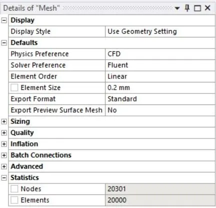
Fig(b). Mesh Details.

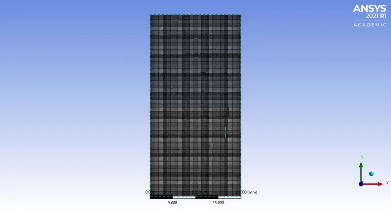
Fig(c). Mesh

3. Setup and Solving (Fluent).

The same parameters of case 1 are used in this case also.

• Time step = 0.005
• No. of time step = 1500

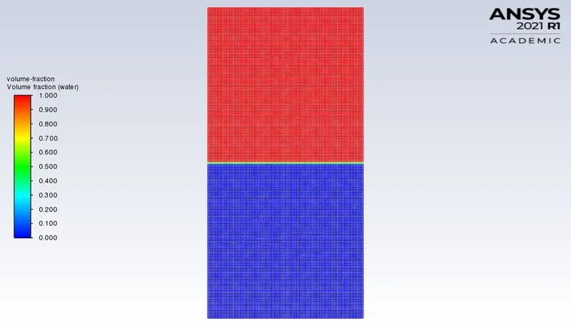
Contour:-

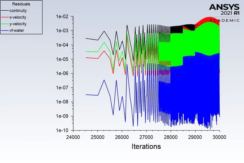
Residuals:-

4. Post-Processing Result.

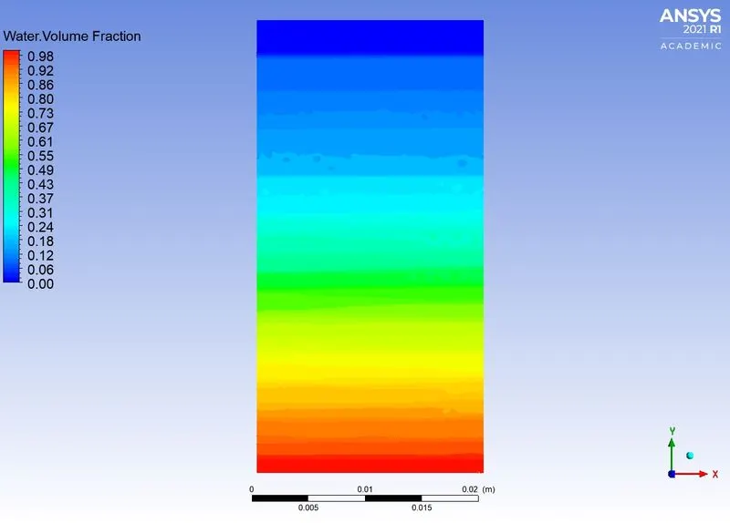
1. Water Volume Fraction contour:-

2. Penetration of heavier fluid into the lighter fluid at different Time steps:-

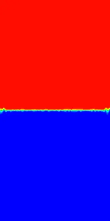
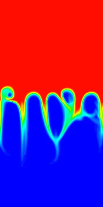
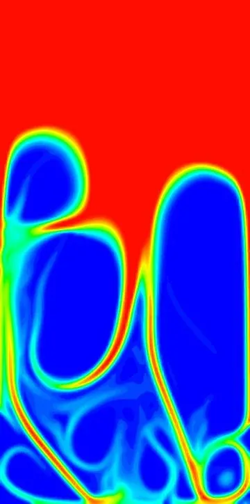
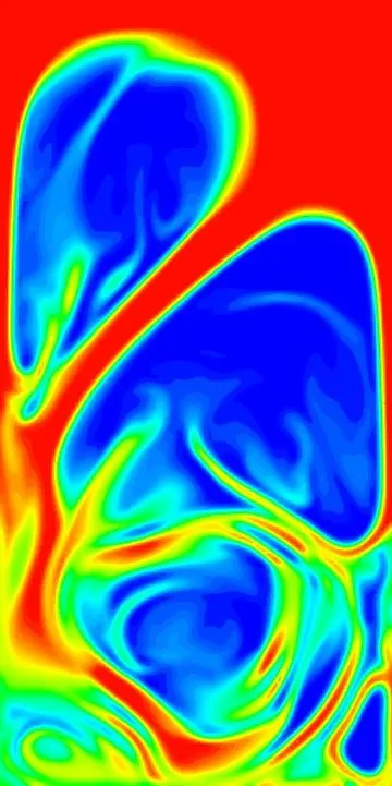
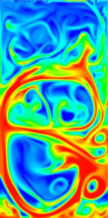
(a) 0.025s (b) 0.075s (c) 0.15s (d) 0.25s (e) 0.5s

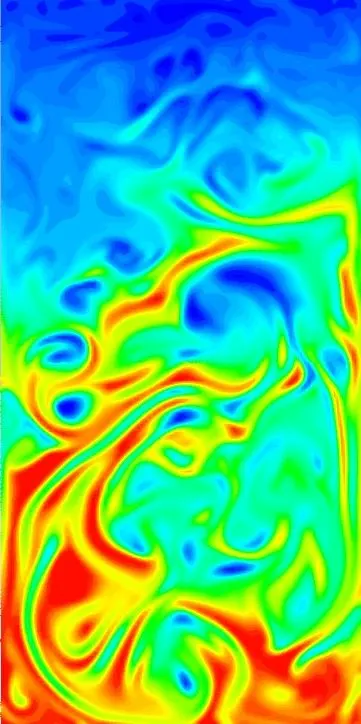
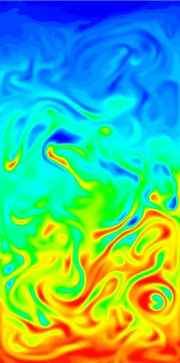
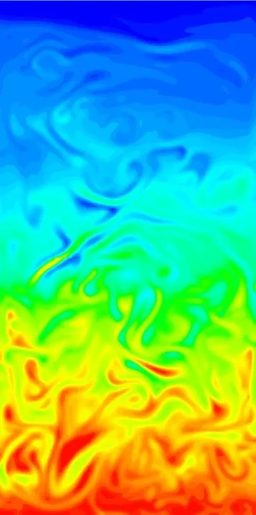
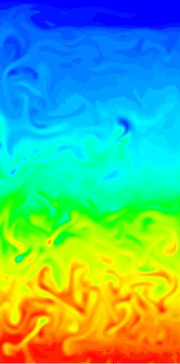
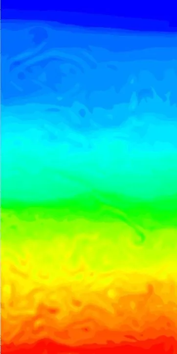
(f) 0.75s (g) 1s (h) 1.25s (i) 1.5s (j) 2s

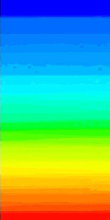
(k)2.5s (l) 3.5s (m) 5s (n) 6.5s (o) 7.5s

3. Animation.

Drive Link - https://drive.google.com/file/d/1Rom8etNPz3HscCPymrTX2CS_JOZ-3G2j/view?usp=sharing

CASE - 3:-

1. Geometry (Spaceclaim).

The geometry is the same as in case-1 and case-2.

Fig(a). Geometry developed in Spaceclaim.

2. Meshing.

• Meshing the geometry with a Refined mesh of 0.2 mm and user-defined material.
• Elements = 20000

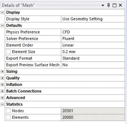
Fig(b). Mesh Details.

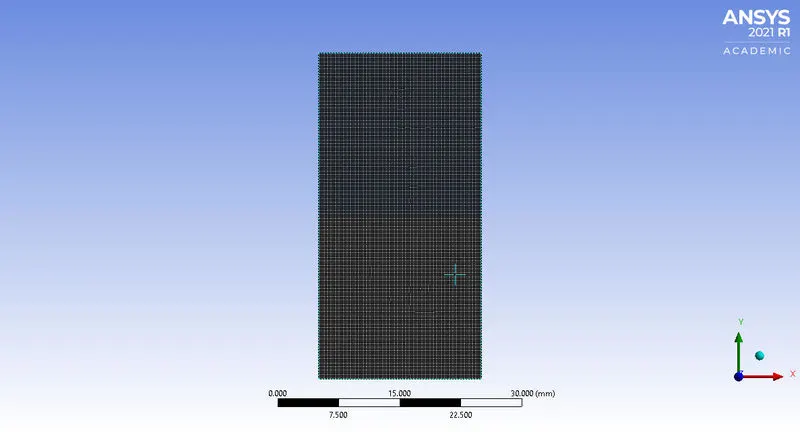
Fig(c). Mesh

3. Setup and Solving (Fluent).

Material:-

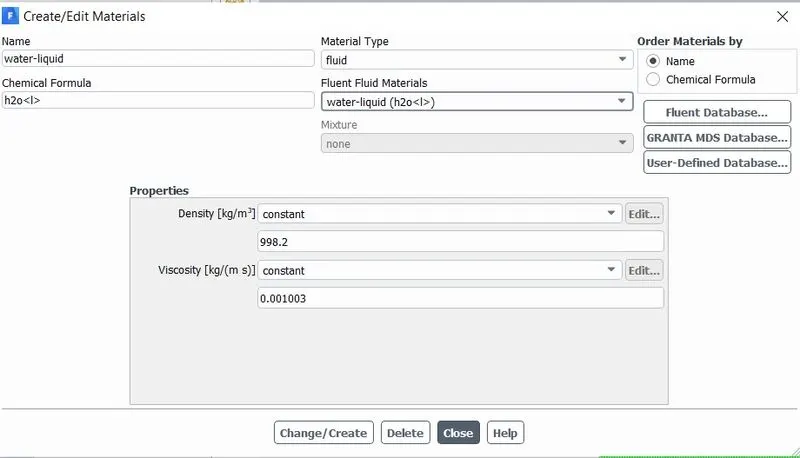
Fig(1). Water is used as a material.

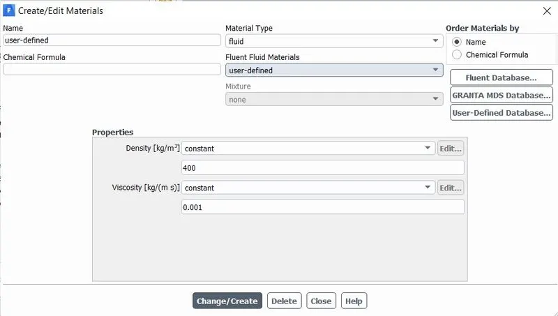
Fig(2). User-defined material is used.

The other procedure is the same as the above two cases.

• Time step = 0.005
• No. of time step = 1500

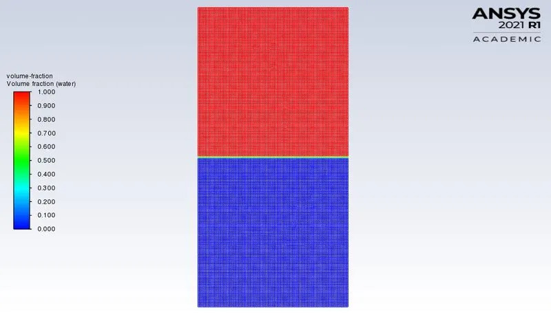
Contour:-

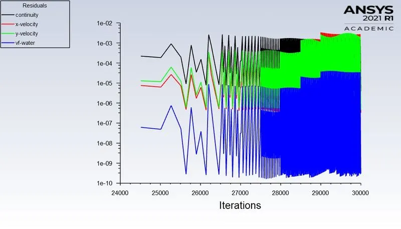
Residuals:-

4. Post-Processing Result.

1. Water Volume Fraction contour:-

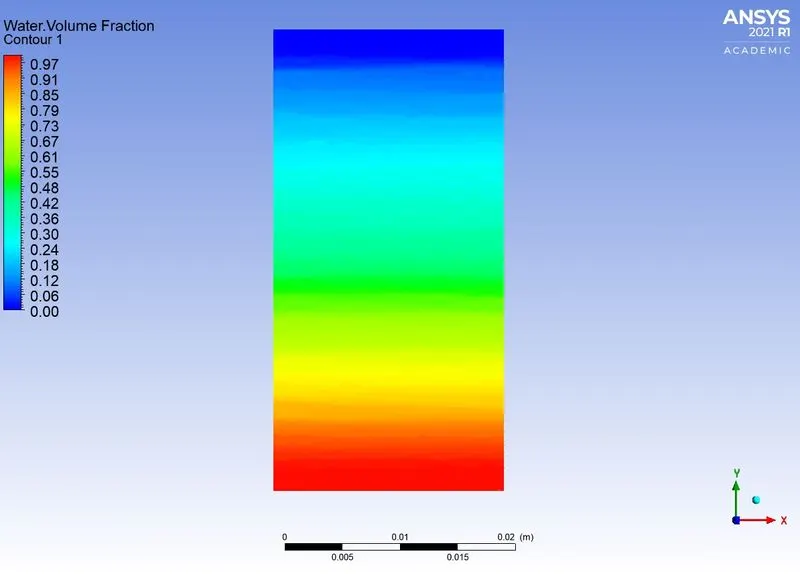
2. Penetration of heavier fluid into the lighter fluid at different Time steps:-

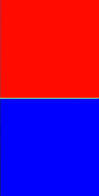
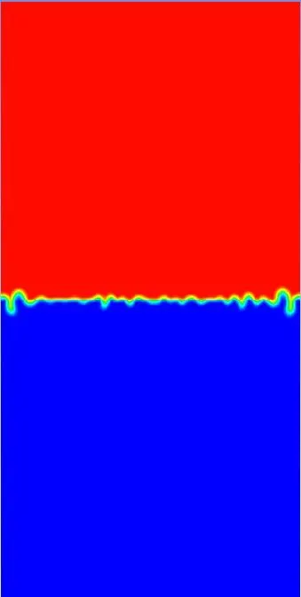
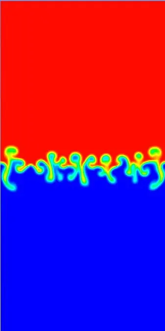
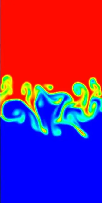
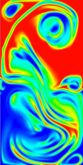
(a) 0.025s (b) 0.125s (c) 0.175s (d) 0.25s (e) 0.5s

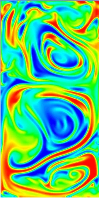
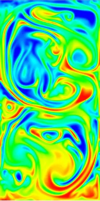
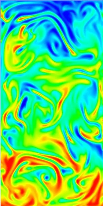
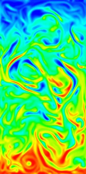
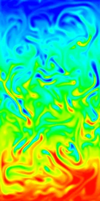
(f) 0.75s (g) 1s (h) 1.25s (i) 1.5s (j) 2s

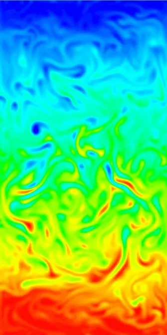
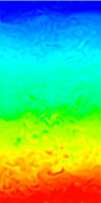
(k) 2.5s (l) 3.5s (m) 5s (n) 6.5s (o) 7.5s

3. Animation.

Drive Link:- https://drive.google.com/file/d/12elBCrabGnShkGXxN9W1CeEW0bVtSXhn/view?usp=sharing

Atwood Number.

`A = (rho_1 - rho_2)/(rho_1 + rho_2)`

Case-1 & Case-2:-

The Atwood number for case-1 and case-2 are the same because the fluid is used.

`A = (998.2-1.225)/(998.2+ 1.225)`

`A = 0.9975`

Case-3:-

`A = (998.2 -400)/(998.2+400)`

`A =0.4278`

Conclusion.

Comparison plot:-

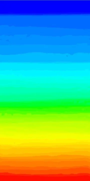
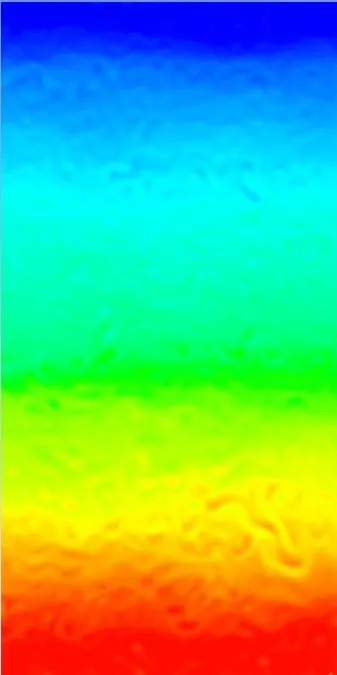
Comparing the plots of four different times of 0.025sec, 1sec, 4sec and 7.5sec.

(a) (b) (c)

Fig(1). Comparison of the 3 cases at Flow time of 0.025sec; (a) Baseline mesh, (b) Refined Mesh, (c) Refined mesh with user-defined material.

(d) (e) (f)

Fig(2). Comparison of the 3 cases at Flow time of 1sec; (d) Baseline mesh, (e) Refined Mesh, (f) Refined mesh with user-defined material.

(g) (h) (i)

Fig(3). Comparison of the 3 cases at Flow time of 4sec; (g) Baseline mesh, (h) Refined Mesh, (i) Refined mesh with user-defined material.

(j) (k) (l)

Fig(4). Comparison of the 3 cases at Flow time of 7.5sec; (g) Baseline mesh, (h) Refined Mesh, (i) Refined mesh with user-defined material.

• From the above plots comparison, the heavier fluid(water) is penetrating the lighter fluid(Air) downwards by gravity.
• The fluid mixing is clear in the Refined mesh and Refined mesh with user-defined material compared to Baseline mesh because of Meshing quality. The finer mesh gives a better result.
• In fig(1) the (a) and (b) plot the water starts penetrating into the air at 0.025sec. But the plot (c) should not start to penetrate at 0.025sec because the density is high in the lower region.
• In fig(2) the (d) and (e) plot the water is reached down in 1sec. But the plot (f) should not reach.
• In fig(3) the (g) and (h) the water settles down in 4 sec and the plot (i) shouldn't settle down.
• From the above plots if the Atwood number is less the penetration of fluid takes more time to settle down.
• The Flow structure of bubbles and globules are quite different both for the variation in meshing and also for the variation in Atwood number.
• The Transient solver is better to capture the fluid flow and can be used to run at smaller time steps compared to a steady-state solver. so that the Steady-state approach might not be suitable for this type of simulation.