Case Study : Rayleigh Taylor Instability

Aim –

• To study the concept of Rayleigh Taylor Instability and its practical CFD models that have been based on the mathematical analysis of Rayleigh Taylor waves.
• To study Rayleigh Taylor Instability simulation for 2 different mesh sizes in addition to baseline and compare the results.
• To study the effect of Atwood number variation on Rayleigh Taylor Instability for all cases.

Criteria Given –

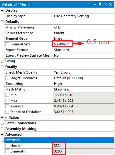
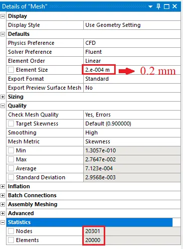
• Baseline Mesh element size – 0.5mm.
• Materials – Phase 1 = Air & Phase 2 = Water/For refined mesh - User-defined material (Density=400 kg/m^3; viscosity = 0.001 kg/m-s).

Introduction –

RTI is phenomenon that occurs at the interface of fluid different density wherein the lighter fluid pushes the heavier fluid due to density difference. It’s a dynamic process wherein the system tries to reduce its combined potential energy.

Theory –

Types of Instability –

• Rayleigh Taylor Instability –

From newton’s law of viscosity., we know that even the fluid cannot resist the slightest shear force. Density is one of the main property of fluid which the force can incorporate with it.

Depending upon density we have lighter fluid like water etc and denser fluid like honey, mercury, oil etc.

Lord Rayleigh observed that when two liquids i.e lighter and heavier fluids are mixed together where the denser fluid is top on the lighter fluid, due to gravity and the density variation the interface of the liquid is not stable. Such as water suspended on oil.

So, the instability of the interface between the different densities of fluid when the lighter accelerated towards the heavier fluid is known as Rayleigh Taylor Instability.

• Ritchmyer-Meshkov Instability –

The Ritchmyer-Meshkov instability arises when shock waves interacts with an interface separating two different fluids. It combines compressible phenomenon such as shock interaction and refraction, with hydrodynamic instability, including nonlinear growth and subsequent transition to turbulence, across a wide range of Mach number.

• Plateau-Rayleigh instability –

The Plateau-Rayleigh instability, often just called the Rayleigh instability, explains why and how a falling stream of fluid breaks up into to smaller packets with the same volume but less surface area. This fluid instability is exploited in the design of a particular type of ink-jet technology whereby a jet of liquid is perturbed into a steady stream of droplets.

• Kevin-Helmholtz instability –

The instability can occur when there is velocity shear in single continuous fluid, or where there is a velocity difference across the interface between two fluids. An example is a wind blowing over water. The instability manifests in waves on the water surface. More generally, clouds, the ocean, Saturn’s bands, and the sun’s corona show thus instability.

CFD model based on mathematical analysis of Rayleigh Taylor waves –

1. Mass diffusion models:

The mass diffusion equation describes the transport of mass and energy due to model viscosity and hence drives actual mixing in the fluids. Even if any configuration in Rayleigh-Taylor unstable, the diffusion process could be responsible for significant mixing if the viscosity is sufficient large.

2. Single fluid model –

• Potential flow model –

This model is valid for all instability changes from early non - linear stage to asymptotic but limited to Atwood number =1. In this model, Single-mode perturbation expands the flow equation to second-order around the bubble tips. Hence, obtaining an ordinary differential equation for bubble velocity.

• Buoyancy drag model –

It is valid for every Atwood number but limited for non-linear stage of instability. It uses ordinary differential equation to evolve the width of mixing layer. The bubble, spikes and amplitude are described by balancing the inertia, buoyancy and drag forces. These models cannot model multiple mixing interfaces, cannot be extended to 2-3 dimensions and as a rule, invalid to address inability to mix, also known as Counter Gradient Transport i.e reduction of total fluid masses within the mixing zone. To address the above problem multi-fluids model have to be used.

• Besnard-Harlow-Rauenzahn (BHR) –

It’s a more advance version if single-fluid model. The BHR model is based on the evolution equations arising from second-order correlations and gradient-diffusion approximations. Using Mass-weighed decomposition, the original BHR model includes full transports equations for the Reynold’s stress, turbulent mass-flux, velocity, density fluctuation and turbulent kinetic energy dissipation rate.

3. Multi-fluid model –

These models use separate set of equation for each fluid in addition to the main flow equations and provide an accurate modeling framework for de-mixing by correctly capturing the relative motion of the different fluid fragments.

The first step fir the development of turbulence models to perform Reynolds averaging of governing equation and the resultant terms.

• Two-equation K-L turbulence model –

The K-L turbulence model involves equations for turbulent kinetic energy K and turbulent length scale L. The starting point of deriving the model equations are the buoyancy-drag models for the self-similar growth of RT instabilities,

• Three equation K-L-a turbulence model –

Three equation model was developed as an extension to the two-equation K-L model including a third equation for the turbulent mass-flux velocity.

• Four-equation model K-L-a-b turbulence model –

Four-equation model was developed as an extension to the three-equation K-L model by including a fourth equation for density-specific volume covariance. The model can accurately reflect the effects of the changes in the density fluctuations.

Procedure –

Problem Setup –

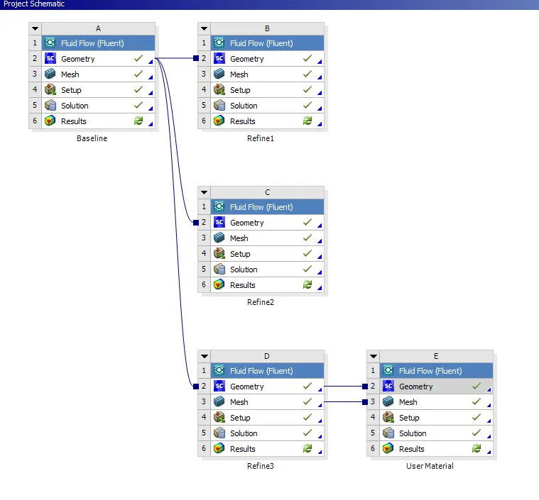
(1) Geometry

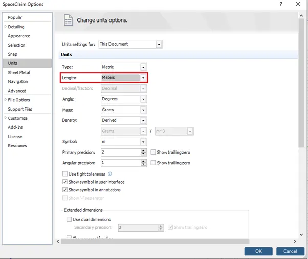
Files → Space Claim Options → Units

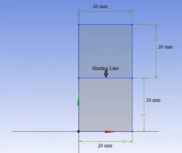
Create a geometry in Space Claim with following dimensions,

Geometry Clip :-

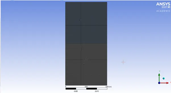
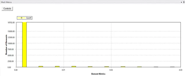
Mesh Generation –

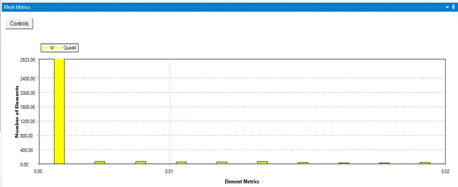
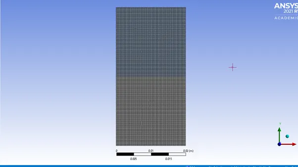
Baseline –

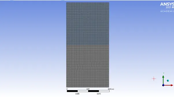
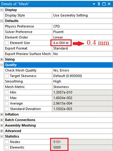
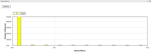
Element Refinement 1 –

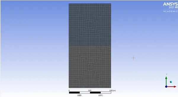
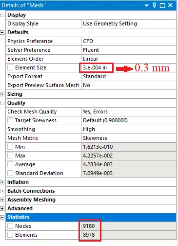
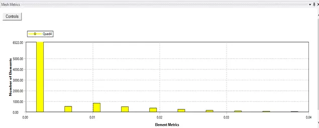
Element Refinement 2 –

Element Refinement 3–

Fluent Setup –

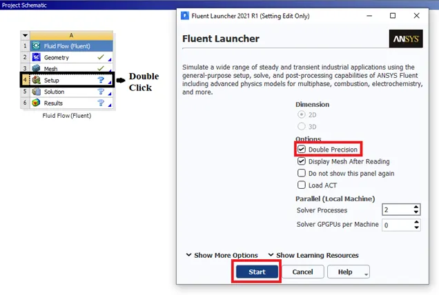
Solution Setup -

1. General → Solver → Pressure-based → Time→ Transient → Gravity → 9.81m/s
2. Models →
3. Viscous → Laminar
4. Multiphase → Volume of fluid → 2 Eulerian Phase → Implicit Scheme

3. Material → Fluid → Add New → Fluent Database → User-Material (In our case user-material has Density=400 kg/m^3; viscosity = 0.001 kg/m-s)
4. Cell Zone Conditions → fff_surface → Fluid → User-material
5. Method → Scheme → Simple
6. Initialize Solution → Hybrid/Standard
7. Results →
8. Create Contour → Phases → Volume Fraction → Field Variable = All Named Selections
9. Activities → Create Animation → Solution Animation → Phase Contour

Results –

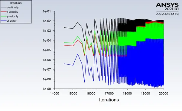
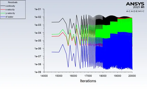
After solving for Time Step = 1000 and 0.005dt (time step size). We arrive at the following inference of solutions and animations respectively for different case comparisons.

Case 1- Baseline Mesh (Air and Water)

Residual Plot -

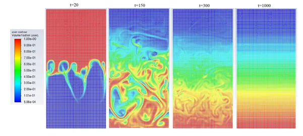
The following animation has been captured at 20, 150, 300 & 1000 frames of animation clip.

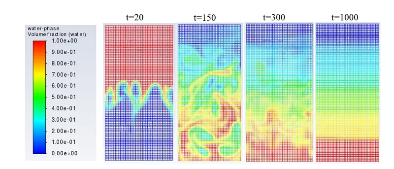
Animation Clip –

Case 2- Refined Mesh 1(Air and Water)

Residual Plot –

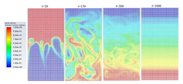
Animation Clip –

Case 3- Refined Mesh 2(Air and Water)

Residual Plot –

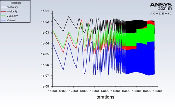
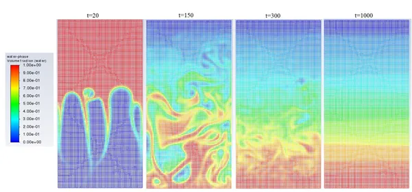
Animation Clip –

Case 4- Refined Mesh 3(Air and Water)

Residual Plot –

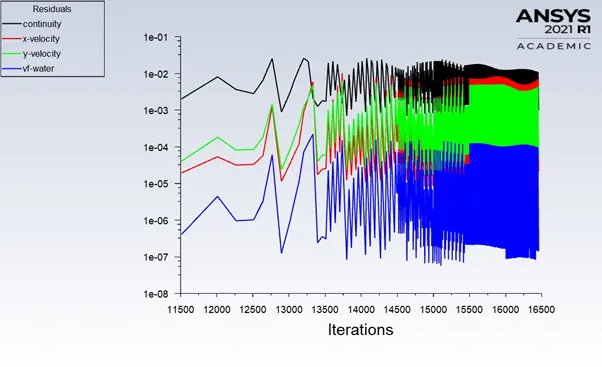
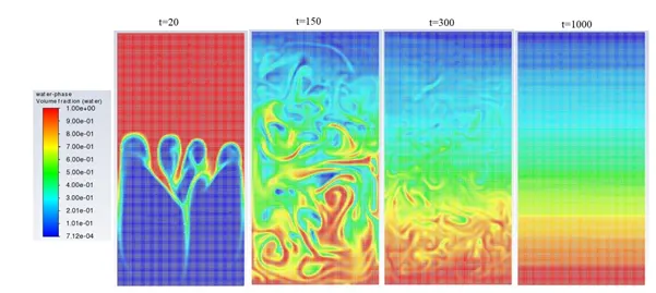
Animation Clip –

Case 5- Refined Mesh 3(Air and User Material)

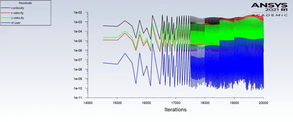
Residual Plot –

Animation Clip –

Observation -

For above cases:

Case 1:

Heavier fluid (Water)

Density 1- 998.2 kg/m^3

Lighter Fluid (Air)

Density 2: 1.225 kg/m^3

Atwood number(A)= 0.996

Case 2:

Heavier fluid (Water)

Density 1: 998.2 kg/m^3.

Lighter fluid (User-defined material)

Density 2: 400 kg/m^3

Atwood number(A)= 0.4276

It’s observed from the simulation that air forms larger bubble when water is burst down the air and forms large bubbles. The Atwood number calculated in case 1 and other cases = 0.42 (approx.).

Inference –

Atwood Number –

Atwood Number(A) is dimensionless number in fluid dynamics used in the study of hydrodynamic instabilities in density stratified flows flow. It’s a dimensionless density ratio defined as:

`A=(rho_1-rho_2)/(rho_1+rho_2)`

Where,

`rho_1`= density of heavier fluid

`rho_2`= density of lighter fluid

Atwood number is an important parameter in the study of Rayleigh-Taylor instability and Richtmyer-Meshkov instability.

In Rayleigh-Taylor instability the penetration distance of heavy fluid bubbles into the light fluid is a function of acceleration time scale.

`A*g*t^2`

Where,

‘g’ is acceleration due to gravity and ‘t’ is time.

• For Atwood number close to 0, RT instability flows take the form asymmetric “finger” of fluid.
• For Atwood number close to 1, the much lighter fluid “below” the heavier fluid takes the form of larger bubble-like plumes.
• Rayleigh-Taylor instability shows three distinct stages namely Linear stability, Bubble formation(rising) and long-term evolution due to bubble merging and mixing.
• For low Atwood number, Bubble and Mushroom head shape is symmetrical, the disturbances or perturbations are linear for a large time.
• In contrast, Atwood number, Bubble and Mushroom head shape is asymmetrical.
• Also, it occurs at rapid rate of acceleration which leads to non-linear growth rate.

Why steady-state approach might not be suitable for above type of simulations?

• The difference between the steady and transient is that you can’t see the small variation of instability.
• The steady-state simulation is performed if we are more concerned about the final state or equilibrium state results.
• In RT- instability CFD models, we are interested in learning about the transition of irregularities that start developing when we pour high dense fluid upon low density fluid under gravity effect so, by using transient solver along the refined mesh of model.
• We can compute the smooth transition of irregularities that takes place at the interface of the fluids.
• The final state results for both the steady-state and transient state will be the same.
• Moreover, in transient we can see the behavior of the solution and every instant such that capturing Bubble, Vortex and Shockwaves.

That’s the reason why transient is more suitable than steady state model.

Conclusion –

Rayleigh-Taylor instability simulation was studied at interface of both fluids having different densities under the influence of gravity and the following observation were made:

• Finer mesh shows formation of bubbles and vortices explicitly.
• Transient state analysis is preferred instead of steady state analysis as we are interested in real-time changes at the interface.
• Atwood number depends of the density of the fluid and ranges from 0 to 1.
• Both Cases have larger Atwood number showing Rayleigh-Taylor instability. Hence matching the simulation results.

Reference -

Numerical Simulations of the Rayleigh-Taylor instability :

https://citeseerx.ist.psu.edu/viewdoc/download?doi=10.1.1.413.7185&rep=rep1&type=pdf