Week 5 - Rayleigh Taylor Instability
AIMS AND OBJECTIVES
- To perform Rayleigh Taylor instability simulation for different mesh sizes with the materials being air and water and compare the results. Also, simulate one case with a user-defined material
- To explain why the steady-state approach is not favored for these types of simulations.
- Talk about some mathematical models based on Rayleigh Taylor analysis and their adaptation for CFD calculations.
- To find the Atwood number for the given cases and effects of variation in Atwood number in the behavior of instability.
Rayleigh Taylor Instability:
It is the instability that happens at an interface between two fluids of different densities suspended together where the lighter fluid pushes through the fluid that is denser. Some of the practical examples include mushroom clouds, atmospheric nuclear explosions, water suspended over oil under gravity, etc.
Some practical models:
- Smoothed-particle hydrodynamics: It is a CFD method used for simulating solid and fluid media. Since it has many advantages over conventional grid-based techniques, it is predominantly used in fluid dynamics. For example, here since particles themselves represent mass, conservation of mass is greatly obeyed. Also, instead of depending on linear systems of equations for solving for pressure, the adjacent particles are relied upon to calculate pressure from their weighted averages. In addition to that, for two-phase interacting fluids, SPH provides a free surface that is independent of boundaries as the particles represent denser fluids and empty space is for a lighter medium. Hence, this technique can simulate physics in real-time.
- Single fluid model: it is a mixture model analysis for two-phase flows where individual fluid phases are assumed to be flowing with mixed properties. It is a five equation model each for mass, momentum, and energy equations in the case of vapor or liquid mixture and two equations for the liquid phase formation or growth.
- Two-phase model: In this model, distinct sets of governing equations are used for liquid and vapor phases. Also, velocity slip between vapor and liquid phase is considered here.
- Discrete Boltzmann model: It is used in phase separation cases in order to study the hydrodynamic and thermodynamic instabilities.
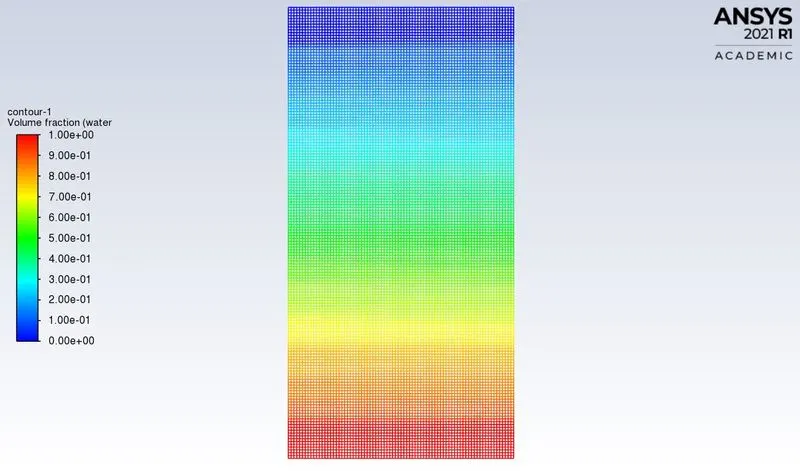
Initial Contour before mixing:
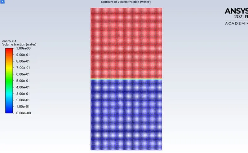
- Case 1
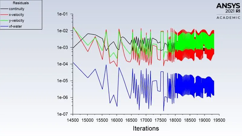
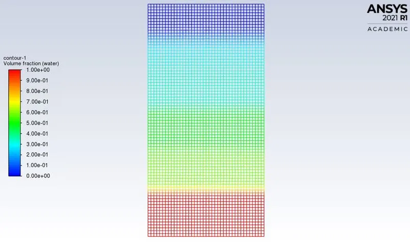
Mesh size = 0.5 mm (baseline mesh)
Convergence Plot:
Volume fraction contour after simulation:
Simulation Animation:
- Case 2
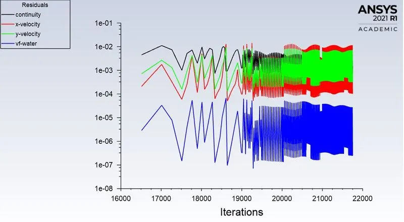
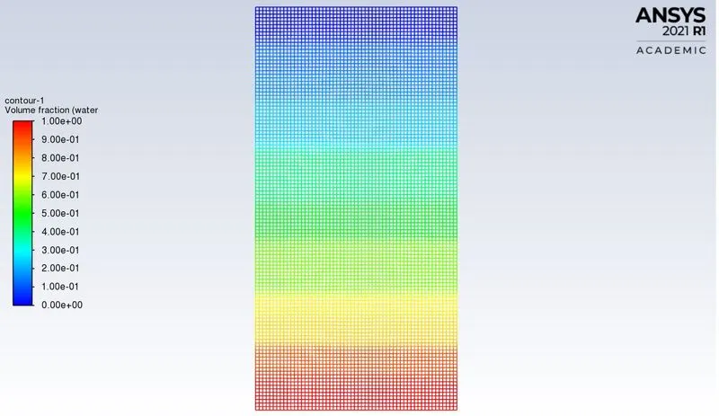
Mesh size = 0.35 mm
Convergence Plot:
Volume fraction contour after simulation:
Simulation Animation:
- Case 3
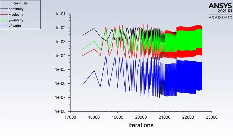
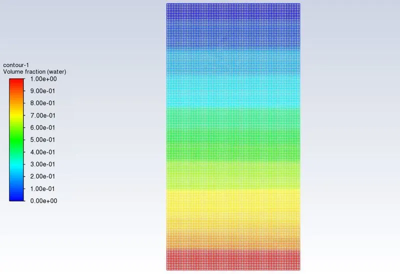
Mesh size = 0.25 mm
Convergence Plot:
Volume fraction contour after simulation:
Simulation Animation:
- Case 4
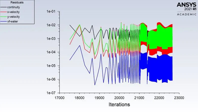
Mesh size = 0.25 mm (user-defined material)
Convergence Plot:
Volume fraction contour after simulation:
Simulation Animation:
Need of transient solver: The steady-state solver essentially gives the final result of the simulation. Here, we are interested to get the time-wise changes happening throughout the simulation. The transient solver gives the time-accurate solutions. Starting from the beginning of instability at the interface between two fluids of different under the gravitational acceleration including capturing instants of the plume formation, vortices, etc until the system reaches a steady-state.
Atwood Number (A):
Atwood number is used in the study of Rayleigh Taylor Instability. If the value of A is close to 1, then it means that the less dense fluid underneath the heavier fluid takes the form of larger plumes. It is basically a dimensionless density ratio.
`A = (rho_1-rho_2)/(rho_1+rho_2)`
where;
`rho_1` = density of the heavier fluid
`rho_2` = density of the lighter fluid
The density of air = 1.225 kg/m³
The density of water = 997 kg/m³
Atwood number, A = (997-1.225)/(997+1.225) = 0.99754 kg/m³
If density of air is 400 kg/m³,
A = (997-400)/(997+400) = 0.42734 kg/m³
Inference:
Here, the water is chosen as heavy fluid and air is less dense fluid. Instabilities can be observed at the interface as the simulation progresses. The physics is well captured and the shocks and irregularities can be well observed when the mesh becomes finer. The Atwood number for the same is calculated to be 0.99754 kg/m³ which is closer to 1 and hence the air pushes through the water upwards to form bubble-like plumes before it is settled. In the second case, the density of the air is increased so that the Atwood number is calculated as 0.42734 kg/m³. Here, the perturbations are found to be relatively symmetrical and the size of plumes started diminishing. Hence, the value of Atwood number conclusively validates the simulation.