Rayleigh Taylor Instability

Aim:

To perform a 2-D Rayleigh-Taylor instability simulation at different mesh refinement and at different atwood numbers.

Theory:

Rayleigh - Taylor instability

The Rayleigh-Taylor instability occurs when a fluid of low density ⍴l, accelerates a fluid of heavy density ⍴h. It occurs in astrophysics, supernova, geophysics, and technology inertially confined fusion among other subjects. The RT mixing rate is the dimensionless coefficient in the equation

h = (𝜶)xAgt2

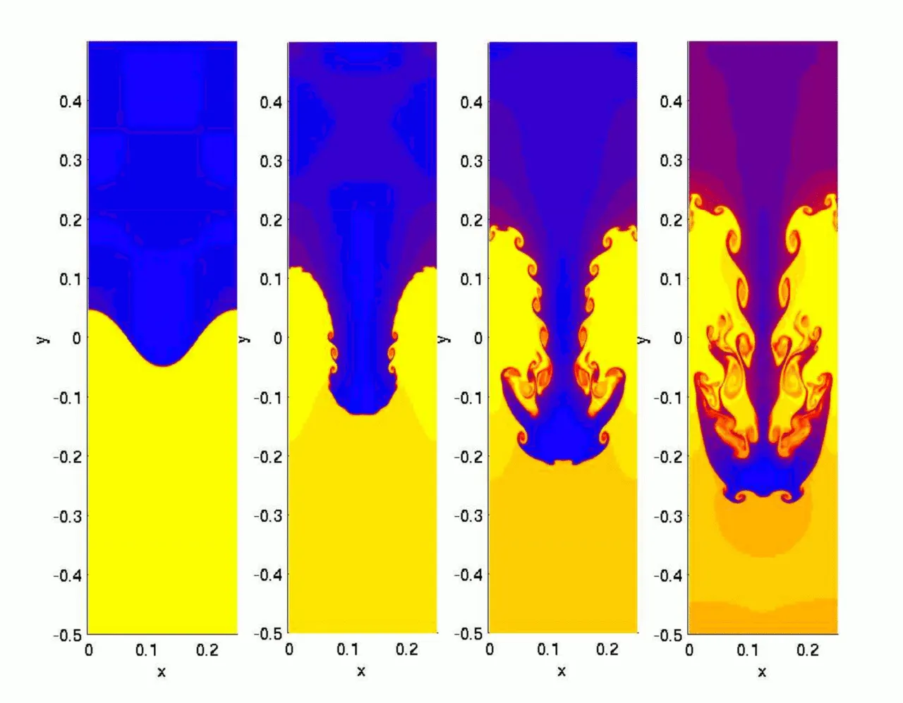
Hydrodynamic simulation of a single "finger" of the Rayleigh–Taylor instability.

for the height h of the bubbles, i.e., the interpenetration distance h of the light fluid into the heavy fluid. Here, A is the Atwood number, g is the acceleration due to gravity and t is the time. Acceptable experimental values for (𝜶) are = 0.063± 0.013

Atwood number

The Atwood number (A) is a dimensionless number in fluid dynamics used in the study of hydrodynamic instabilities in density stratified flows. It is a dimensionless density ratio defined as

A=(⍴h)−(⍴l) /(⍴h)+(⍴l)

Atwood number is an important parameter in the study of Rayleigh–Taylor instability and Richtmyer–Meshkov instability. In Rayleigh–Taylor instability, the penetration distance of heavy fluid bubbles into the light fluid is a function of acceleration time scale, Agt2

Stages of development and eventual evolution into turbulent mixing

The evolution of the RTI follows four main stages. In the first stage, the perturbation amplitudes are small when compared to their wavelengths, the equations of motion can be linearized, resulting in exponential instability growth. In the early portion of this stage, a sinusoidal initial perturbation retains its sinusoidal shape. However, after the end of this first stage, when non-linear effects begin to appear, one observes the beginnings of the formation of the ubiquitous mushroom-shaped spikes (fluid structures of heavy fluid growing into light fluid) and bubbles (fluid structures of light fluid growing into heavy fluid). The growth of the mushroom structures continues in the second stage and can be modeled using buoyancy drag models, resulting in a growth rate that is approximately constant in time. At this point, nonlinear terms in the equations of motion can no longer be ignored. The spikes and bubbles then begin to interact with one another in the third stage. Bubble merging takes place, where the nonlinear interaction of mode coupling acts to combine smaller spikes and bubbles to produce larger ones. Also, bubble competition takes place, where spikes and bubbles of smaller wavelengths that have become saturated are enveloped by larger ones that have not yet saturated. This eventually develops into a region of turbulent mixing,which is the fourth and final stage in the evolution. It is generally assumed that the mixing region that finally develops is self-similar and turbulent, provided that the Reynolds number is sufficiently large.

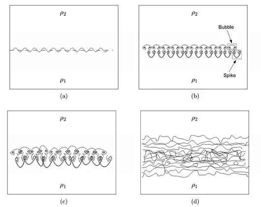
(a) Small wavelength perturbations at the interface

(b) Growth of the ubiquitous mushroom shaped spikes (fluid structures of heavy fluid into light fluid) and bubbles (fluid structures of light into heavy fluid)

(c)The fluid structures interact due to bubble merging and competition

(d)A mixing region is developed.

Note: ρ2 = heavy fluid and ρ1 = light fluid.

Classification of models:

Mass diffusion model:

To model the mixing of compressible miscible fluids with mass diffusion, the conservation equations take the form

Single fluid model:

• Potential flow model

An elementary description of RT instability can be given in terms of potential flow theory. It provides a well-known framework for the study of surface modes and has been the basis of many classical stability results. Important aspects of this approach are that the most severe interfacial perturbations can be isolated by this model, giving usually an upper bound on instability growth. Furthermore, it pertains to nonlinear evolution in a relatively simple manner.

• Buoyancy-Drag model

is a simple model, based on ordinary differential equations, for estimating the growth in the width of a turbulent mixing zone at an interface between fluids of different densities due to Richtmyer–Meshkov and Rayleigh–Taylor instabilities. The model is calibrated to give the required self-similar behavior for mixing in simple situations. However, the early stages of the mixing process are very dependent on the initial conditions and modifications to the Buoyancy-Drag model are then needed to obtain correct results.

• Besnard-Harlow-Rauenzahn(BHR)

The BHR model is based on the evolution equations arising from second-order correlations and gradient-diffusion approximations. Using a mass weighted averaged decomposition, the original BHR model includes full transport equations for the Reynolds stresses, turbulent mass-flux velocity, density fluctuations and the turbulence kinetic energy dissipation rate.

Multi-fluid model:

• The k-L turbulence model:

It’s the model where k is the turbulent kinetic energy and L represents the turbulent eddy scale length, is a two-equation turbulence model that is used to simulate turbulence induced by Rayleigh-Taylor (RT) and Richtmyer Meshkov (RM) instabilities. The starting point for deriving the model equations are the buoyancy-drag models for the self-similar growth of RT instabilities.

• Three-equation K-L-a turbulence model:

The three equation model was developed as an extension to the two-equation K-L model by including a third equation for the turbulent mass-flux velocity.

• Four-equation K-L-a-b turbulence model:

The four equation model was developed as an extension to the three-equation K-L model by including a fourth equation for density-specific volume covariance. The model can accurately reflect the effects of the changes in the density fluctuations.

Calculation:

Atwood number:

For simulation involving air and water:

A=(⍴h)−(⍴l) /(⍴h)+(⍴l) = (998.2-1.225)/(998.2+1.225) = 0.997

For simulation involving user-defined material and water:

A=(⍴h)−(⍴l) /(⍴h)+(⍴l)= (998.2-400)/(998.2+400) = 0.427

Procedure:

• Preparation of geometry

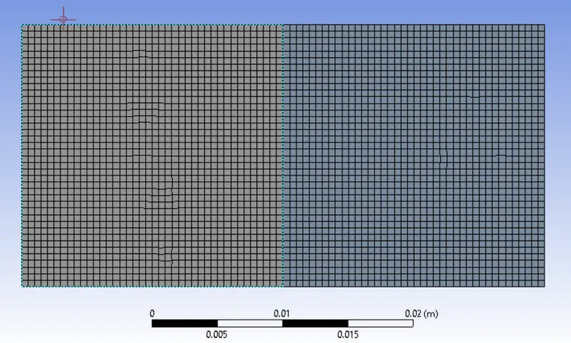
The geometry is essentially two squares , one on top of another of side 20 mm. The top square has been named 'water' and bottom square 'air' . The common edge between the domains was shared using share tool in Workbench. The created geometry is depicted below:

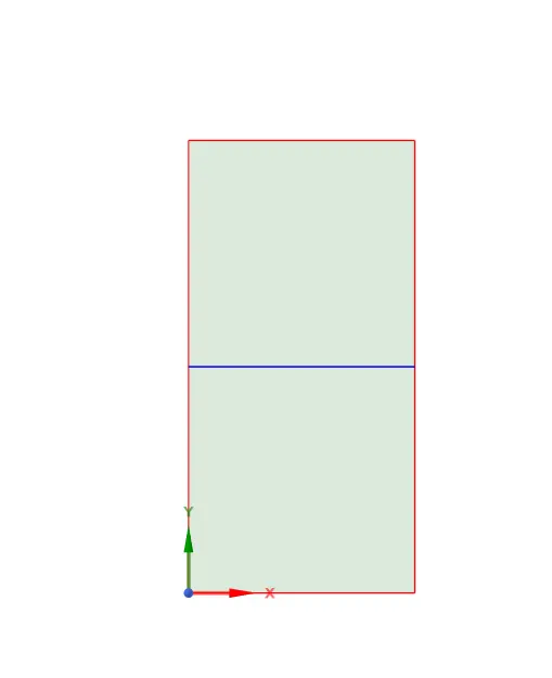
The topology faces between the two squares are shared under workbench>share.

• Meshing

Baseline mesh element size = 0.5 mm

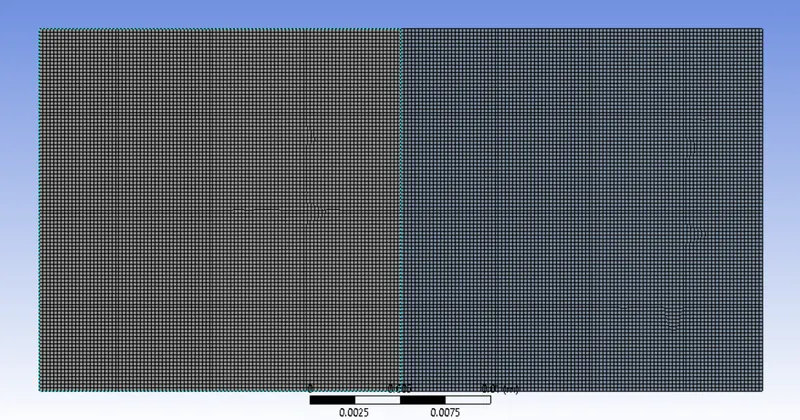
Refined mesh element size = 0.2 mm

• Solving

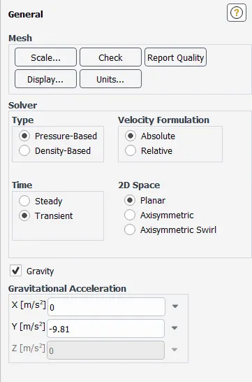
General setting of solver -

• Pressure based
• Transient solver
• Absolute velocity formulation
• Gravity of value -9.81 m/s^2

Viscous model - Laminar

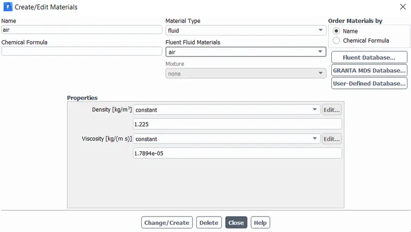
Material properties of

• air

• water

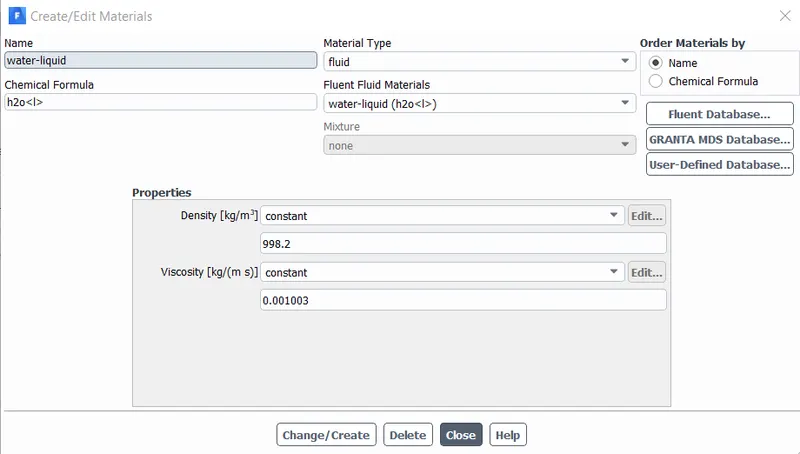
• user-defined material

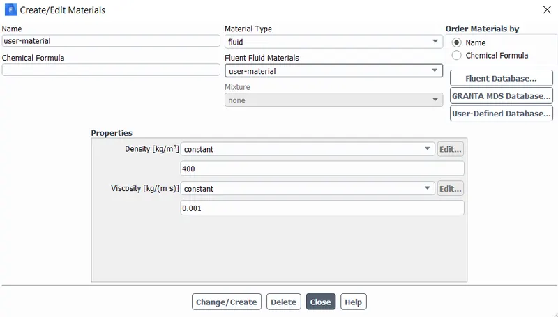
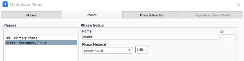
Multi-phase model properties:

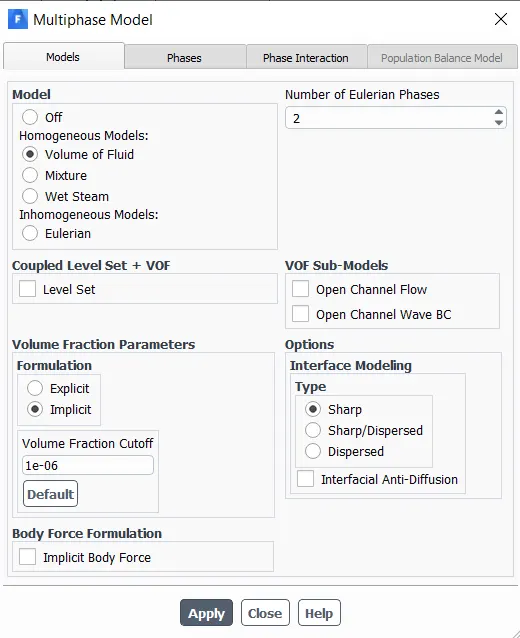
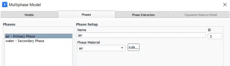
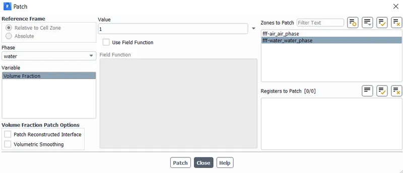
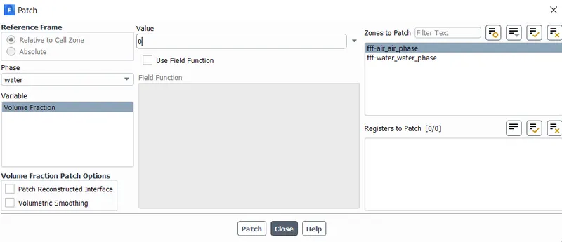
After Standard Initialization ,we have to patch both the domains to the respective materials, wherein we provide a volume-fraction value of 1 to water and 0 to air and user-defined material.

Enable auto save option to save results after every 5 iterations and then solve for 1500 Time steps with 0.05 dt (time step size).

Observation:

Coarse mesh results:

Atwood number = 0.997

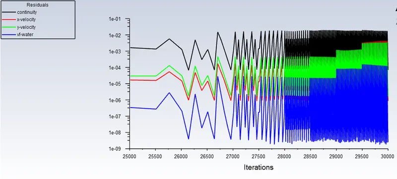
Residuals:

Link to instability flow animation:

https://drive.google.com/file/d/1mqu0toPhxKNi6Jg0JARQdw0KDFjG36hu/view?usp=sharing

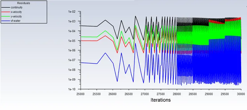
Refined mesh results:

Atwood number = 0.997

Residuals:

Link to instability flow animation:

https://drive.google.com/file/d/1KzZEBRerpkx0YBPFq5OWGUXbnOJMHh7a/view?usp=sharing

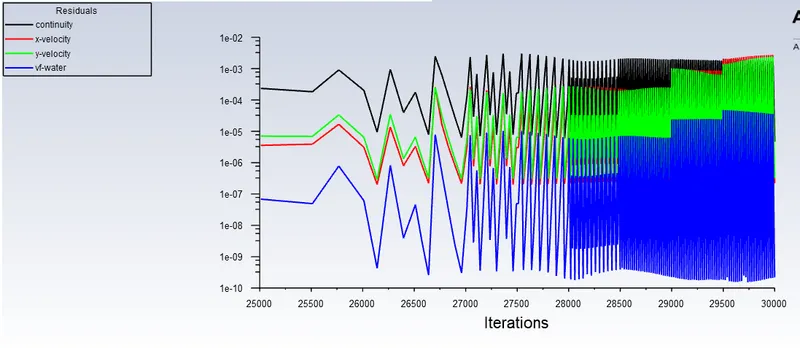
Simulation with user defined-material:

Atwood number = 0.427

Residuals:

Link to instability flow animation:

https://drive.google.com/file/d/1BtlVn3nyQL27VXdOd2U7fsL8t8wccSk-/view?usp=sharing

Inference:

• Finer mesh captures the instability better than the coarse mesh
• Finer mesh takes more computational resources, hence more time consuming but produces results with better accuracy.
• Since the simulation involves capturing instabilities that change in an unpredictable manner over a period of time, transient approach is better suited as compared to steady state approach.
• Hence the steady state approach does not predict the flow and bears incorrect results at the end.
• For low Atwood number, bubble and mushroom head shape is relatively more symmetrical, the perturbation growth are linear for a longer time.
• For large Atwood number, bubble and mushroom head shape is less symmetrical, also it occurs very rapidly at an accelerated rate which leads to a non linear growth rate of perturbations.

Conclusion:

2-D Rayleigh-Taylor instability simulation was performed at different mesh refinement and at different atwood numbers.