Week 5 - Rayleigh Taylor Instability

AIM: To conduct some practical CFD models that have been based on the mathematical analysis of Rayleigh Taylor waves.

OBJECTIVE:

1. Perform the Rayleigh Taylor instability simulation for 2 different mesh sizes with the base mesh being 0.5 mm.
2. Observe the differences in the animation and explain the effect of mesh size on simulation.
3. Explain why a steady-state approach might not be suitable for these types of simulation.
4. Run one more simulation with water and user-defined material(density = 400 kg/m³, viscosity = 0.001 kg/m-s) for refined mesh.
5. Define the Atwood Number. Find out the Atwood number for both the cases and explain how the variation in Atwood number in the above two cases affects the behavior of the instability.

THEORY AND EXPLANATION:

RAYLEIGH TAYLOR INSTABILITY(RTI):

Rayleigh Taylor Instability (RTI) is a phenomenon that occurs at the interface of fluids of different densities wherein the lighter fluid pushes the heavier fluid due to the density difference. It is a dynamic process wherein the system tries to reduce its combined potential energy. Initially, the system is in a state of hydrostatic equilibrium, in which the heavier fluid(ex: water) sits a top a lighter fluid(ex: air) in a constant gravitational field. As the RTI develops, the initial perturbations progress from a linear growth phase, eventually developing "plumes" flowing upwards(in the gravitational buoyancy sense) and "spikes" falling downwards. In the linear phase, equations can be linearized and the amplitude of perturbations is growing exponentially with time. In the non-linear phase, the perturbation amplitude is too large for the non-linear terms to be neglected. In general, the density disparity between the fluids determines the structure of the subsequent non-linear RT instability flows (assuming other
variables such as surface tension and viscosity are negligible here). Examples include supernova, water suspended atop oil, mushroom clouds formed due to volcanic eruptions.

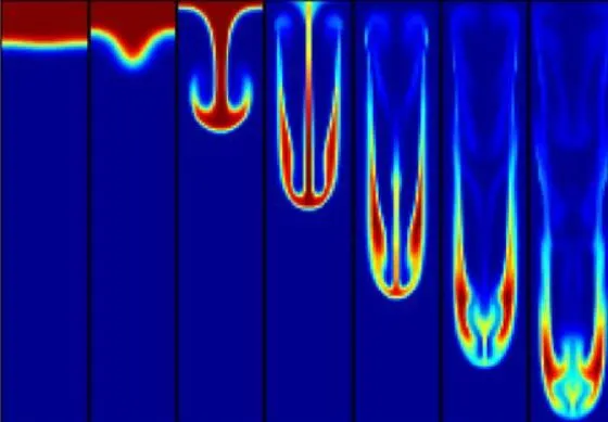
PRACTICAL CFD MODELS:

SPH method(Smoother particle hydrodynamics) Smoothed-particle hydrodynamics (SPH) is a computational method used for simulating the mechanics of continuum media, such as solid mechanics and fluid flows. Smoothed-particle hydrodynamics is being increasingly used to model fluid motion as well. This is due to several benefits over traditional grid-based techniques. First, SPH guarantees conservation of mass without
extra computation since the particles themselves represent mass. Second, SPH computes pressure from weighted contributions of neighboring particles rather than by solving linear systems of equations. Finally, unlike grid-based techniques, which must track fluid boundaries, SPH creates a free surface for two-phase interacting fluids directly since the particles represent the denser fluid and space represents the lighter fluid.

SINGLE-FLUID MODEL:

A typical approach used for the analysis of two-phase flows is a mixture model, i.e. the individual fluid phases are assumed to behave as a flowing mixture described in terms of the mixture properties. The applied single-fluid model is a five-equation model consisting of the mass, momentum, and energy equations for a vapor/liquid mixture, and two equations describing the formation and growth of the liquid phase.

TWO-FLUID MODEL:

In the two-fluid model, separate sets of the governing equation for the vapor and liquid phases have been used. The interaction between the droplets and the heat exchange between the liquid phase and the solid boundary is not modeled here as well. Additionally, the velocity slip between the vapor and the liquid phase is in this model taken into account.

TURBULANCE MODEL:

Turbulence models are needed to predict the average mixing behavior inflows that are on average one- or two-dimensional. The approach to the construction of the tile turbulence model is guided by experimental behavior. The equations governing turbulent flows can only be solved directly for simple cases of flow. For most real-life turbulent flows, CFD simulations use turbulent models to predict the evolution of turbulence. These turbulence models are simplified constitutive equations that predict the statistical evolution of turbulent flows.

PROCEDURE:

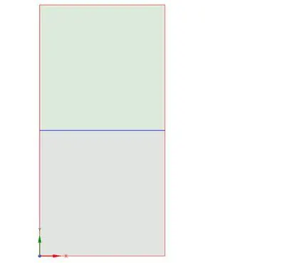
1. Create a square of 20mm*20mm.Use Pull tool in order to create a surface.

2. Then naming the below square as air and above square as water in 2 different components.

3. And share the topology for a perfect intersection between both surfaces.

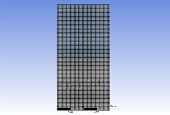
4. Overall element size is 0.5mm.

5. The general time setting was changed to transient and gravity was introduced along y axiz.

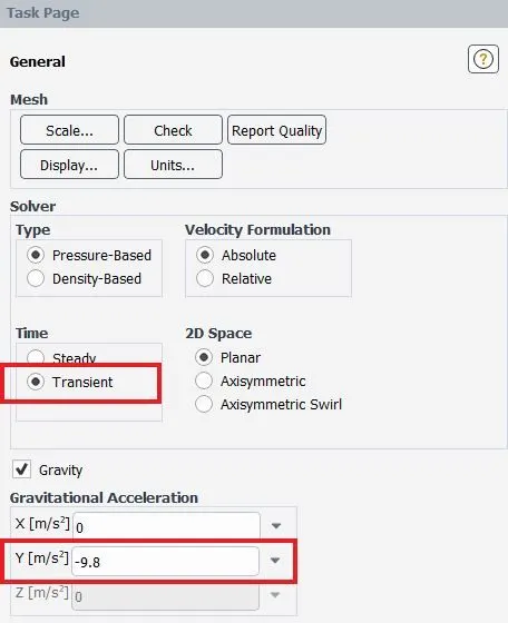
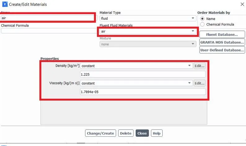
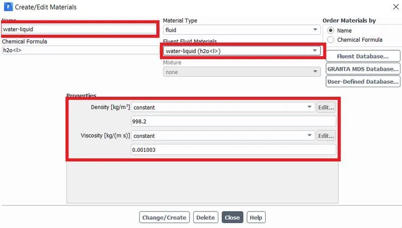
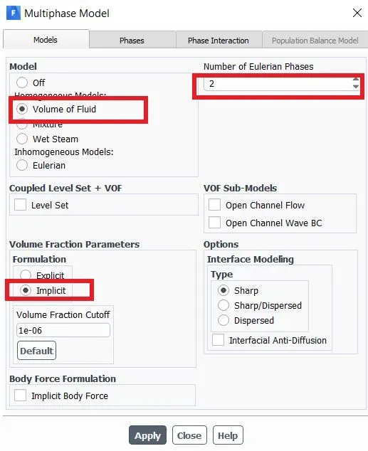
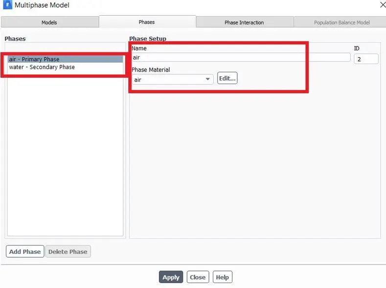
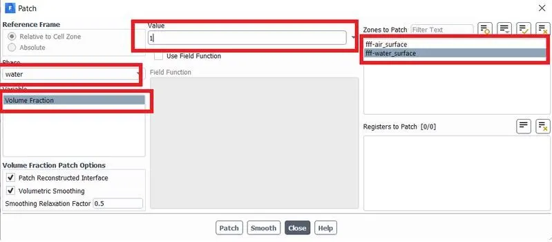
The solution was run for 1500 timesteps with 0.005 timestep size.

RESULTS:

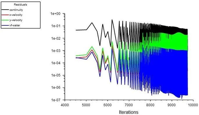
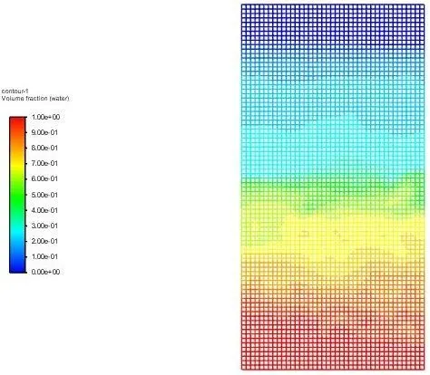
CASE1: For mesh size = 0.5mm, Air + Water

RESIDUALS PLOT:

PHASE CONTOUR:

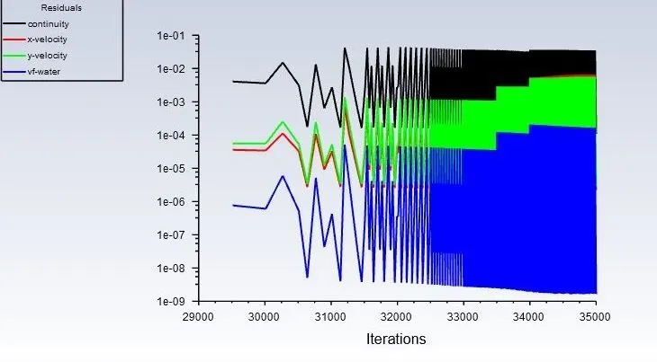
CASE2: For mesh size = 0.1mm, Air + Water

RESIDUALS PLOT:

PHASE CONTOUR:

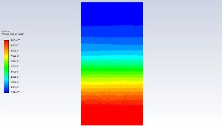
CASE3: For mesh size = 0.1mm, User material + Water

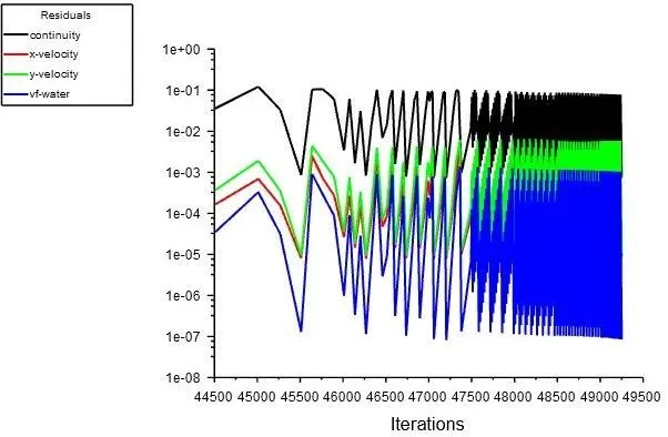
RESIDUALS PLOT:

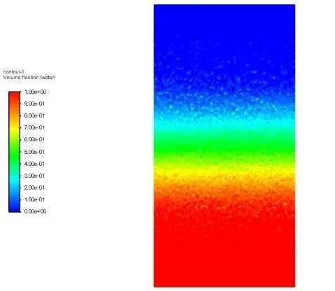
PHASE CONTOUR:

Steady-state simulation is not suitable because:

1. We know that a steady-state simulation is a time-independent approach.

2. Based on the simulation, we know that there is high turbulence, and the flow change occurs between very small time variations. It is impossible to capture in steady-state simulation.

3. Also, the steady-state solver ignores the time differential terms involved in the simulation. Therefore, even if it can capture the state of equilibrium, it doesn't capture the non-linearities in the simulation precisely.

Atwood number:

The Atwood number (A) is a dimensionless number in fluid dynamics used in the study of hydrodynamic instabilities in density stratified flows. It is a dimensionless density ratio defined as:

A = ρ₁ - ρ₂ / ρ₁ + ρ₂

where

ρ₁ = Density of heavier fluid

ρ₂= Density of lighter fluid

In case 1&2:

ρ₁ = 1000 and ρ₂ = 1.225

A= 1000-1.225/1000+1.225 = 0.9975

In case 3:

ρ₁ = 1000 and ρ₂ = 400

A= 1000-400/1000+400= 0.4285

We can observe that as the Atwood number decreases, the time taken to reach steady state also decreases. In case 3, the user defined fluid was much denser(or more viscous ) hence the formation of instabilities were quite low and reached a steady state quite fas compared to other 2 cases since the difference between density of the 2 fluids are less. We cannot use steady state approach for these types of simulations as we need to study the change with respect to time , which is possible only in transient simulations.

CONCLUSION:

1. From the above cases, we observe that finer mesh captures the instability better than the coarse mesh, but it takes more time for the heavier fluid to settle down. As computational time is long but produces results with better accuracy.

2. Since the simulation involves capturing instabilities that are changing in an unpredictable manner as a function of time, the transient approach is preferred over the steady-state approach.

3. The Atwood no validates the CFD simulation as it is observed. In the case of water and air mixing, bubble formation takes place, whereas in the other case no bubble takes place.