Week 5 - Rayleigh Taylor Instability

AIM : To simulate Rayleigh Taylor instability and to understand CFD modelling method of VOF ( Volume of Fluid) for multiphase flows

THEORY : In fluid mechanics, Multiphase flow is the simultaneous flow of two or more phases . This could be fluid-solid, solid-solid, fluid-fluid. A few examples would be

• Oil and water separation in pipelines
• Boiling and condensation in heat exchangers
• bubbly flow in chemical reactors

The multiphase flow can be broadly categorized into two

• dispersed flow , which includes finite particles like bubbles dispersed in a continuous phase
• separated flows which includes two or more phases separated by interfaces.

A few examples of multiphase flows are given below

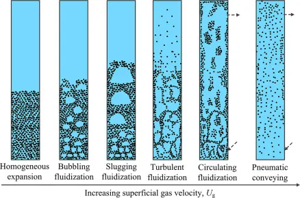
Fluidized bed simulations come under the category of multiphase flows as the simulations are done to simultaneously solve two phase like a gas solid fluidized bed. Here the two phases are seen as inter penetrating continua and the modelling approach used is Eulerian Eulerian CFD simulations.

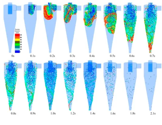
Cyclone separators are used in industries to remove particulates from gas streams. When air enters the separators, they are spined causing the particles to be removed by centrifugal forces.

DPM methods ( discrete Phase models) is commonly used for modelling such flows.

There are various other modelling strategies that capture multiphase flows well. They include immersed boundary method, Level Set, Front tracking etc. But in this assignment, the main focus will be on VOF( volume of fluid).

VOLUME OF FLUID

The Volume of Fluid (VOF) method is a numerical technique used in Computational Fluid Dynamics (CFD) to track and model the interface between immiscible fluids, such as water and air, within a computational domain. It is particularly effective in simulating multiphase flows, including free surface flows, sloshing, bubble dynamics, and phenomena like the Rayleigh-Taylor instability. Applications of the VOF method include studying wave dynamics, predicting fluid behavior in microfluidic devices, and analyzing liquid-gas interactions in industrial processes. Pros of the VOF method include its ability to handle complex, highly deformable interfaces and its efficiency in conserving mass without requiring a mesh specifically for the interface. However, cons include challenges in accurately capturing small-scale interface details and potential numerical diffusion, which can lead to smeared interfaces.

1.What are some practical CFD models that have been based on the mathematical analysis of Rayleigh Taylor waves? In your own words, explain how these mathematical models have been adapted for CFD calculations.

Rayleigh Taylor Instability or RTI is a fluid dynamics phenomenon that occurs at the interphase between two fluids, where the fluid on top is denser than the one below it. This leads to an unstable interface and complex wave like patterns/structures. RTI study is quite crucial as it plays a very important role in understanding stability dynamics in fluids , both in natural and man-made phenomenon. A few examples would be

• Supernova and star formation
• Turbulence and mixing
• weather patterns and ocean currents
• Volcanic eruptions

The study of RTI is essential to understanding mixing of fluids. CFD techniques have been implemented to simulate such flows. A few examples are mentioned and explained below :

LINEAR STABILITY ANALYSIS MODELS :

• These models are based on Linear Stability theory where small perturbations are analyzed at the interface of the fluids .
• It involves solving the Navier Stokes equation considering the initial perturbation's growth rate.
• In CFD , it helps in understanding the early stages of instability.

BUOYANCY DRIVEN MODELS :

• These models are from the momentum equations where the buoyancy term is very crucial. This instability arises from the differences in densities which is included in the equation.
• In CFD , the buoyancy term is already included in the Navier stokes equation using a body force term.
• The model tracks how the denser fluid will move through the lighter fluid.

INTERFACE TRACKING TECHNIQUES

• Mathematical models like Level Set or VOF are used to track the interface of the liquids in evolving time.
• CFD simulations use these techniques to accurately track the complex, time-dependent deformation of the interface between fluids. VOF and level-set methods are particularly effective for capturing the highly non-linear and chaotic shapes that develop during RTI.
  

2. Perform the Rayleigh Taylor instability simulation for 2 different mesh sizes with the base mesh being 0.5 mm. Compare the results by showing the animations( Attach them from your google drive). Observe the differences in the animation and explain the effect of mesh size on simulation. Also, explain why a steady-state approach might not be suitable for these types of simulation.

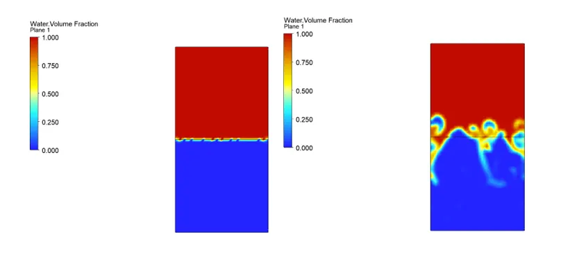
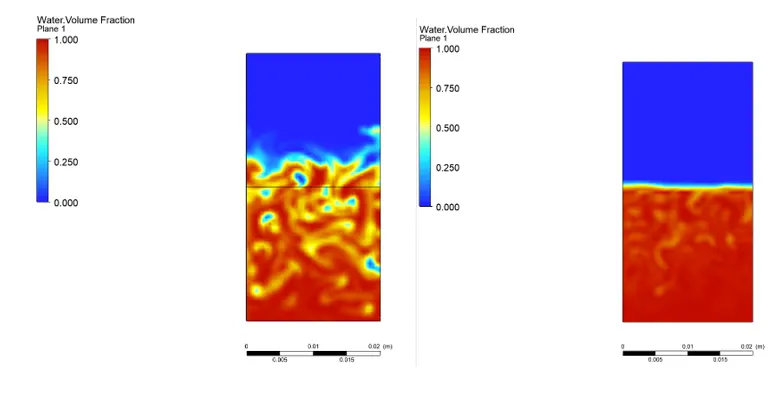
CASE 1: Course mesh with base size of 0.5mm

The contour plots are given below

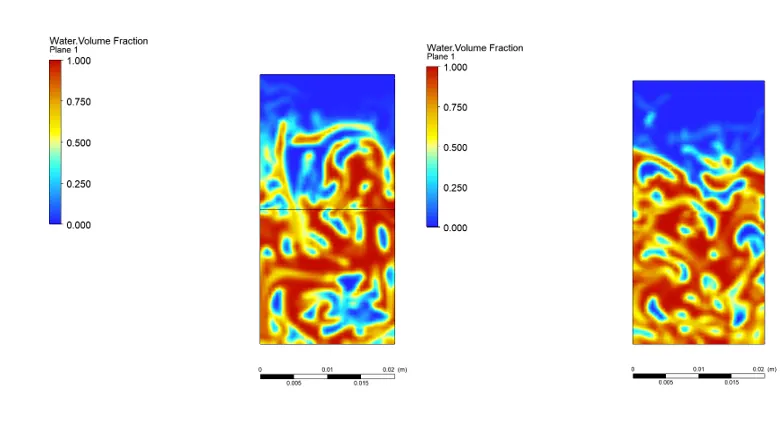
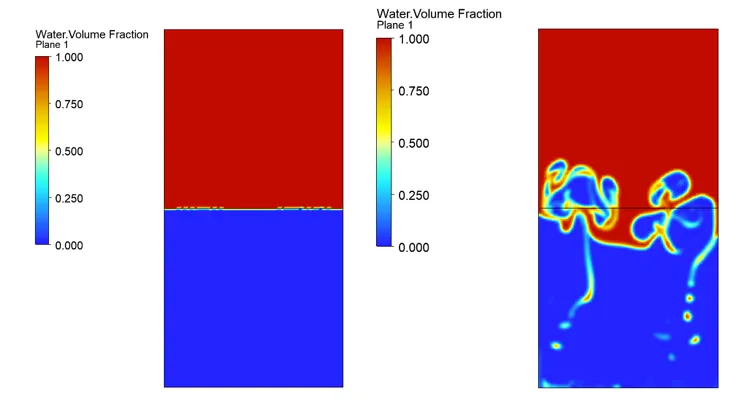
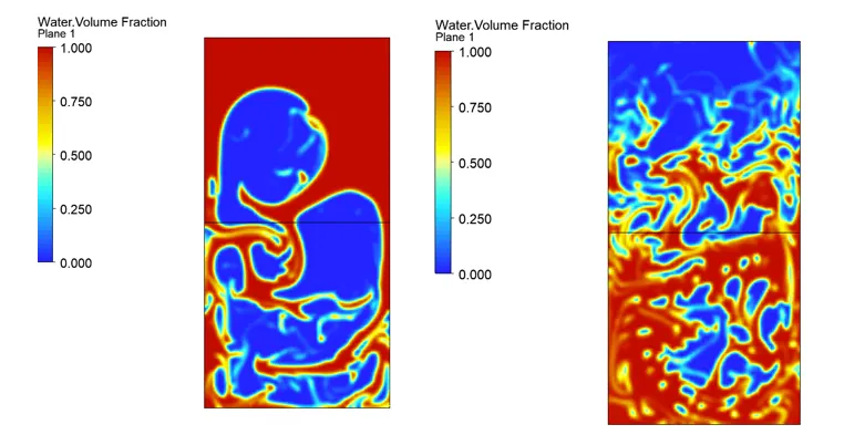
CASE 2 : The simulation was run for water and air, with fine mesh . The contour plots at different time periods are given below

3.Run one more simulation with water and user-defined material(density = 400 kg/m3, viscosity = 0.001 kg/m-s) for refined mesh.

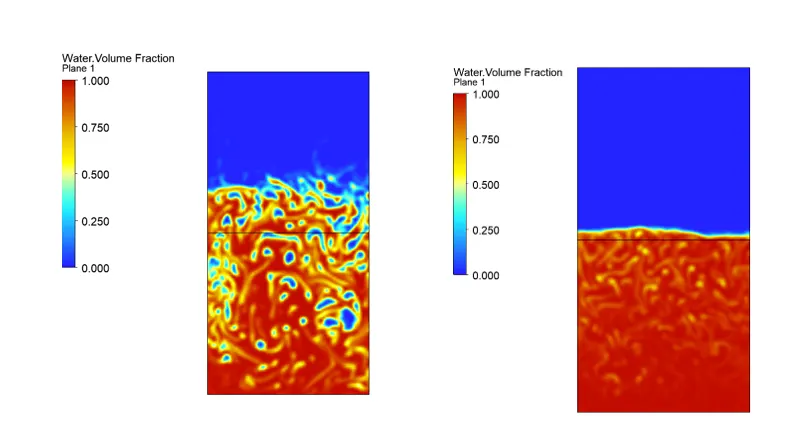
The simulations were run for water and user defined material, and similar plots are given below

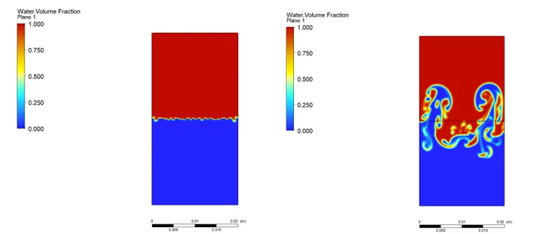
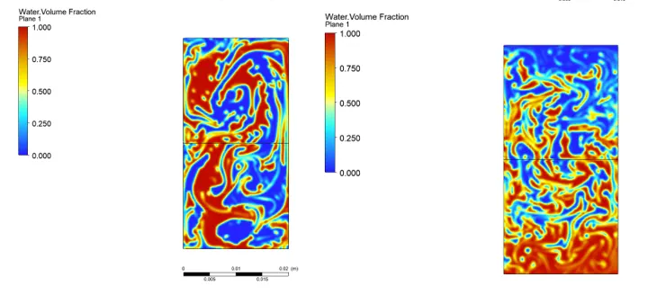
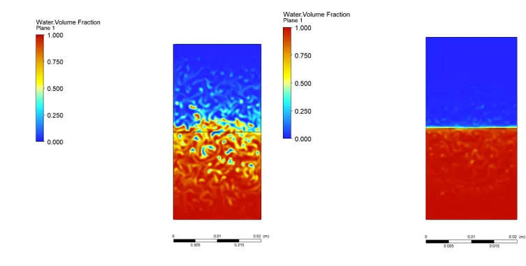
It can be observed from the contour plots that a finer mesh is able to capture the instabilities with much greater accuracy. But if the mesh is fine , the simulation duration is higher which is expected. Here, since we need to study how the instabilities evolve as a function of time, we need a transient simulations.

3. Define the Atwood Number. Find out the Atwood number for both the cases and explain how the variation in Atwood number in the above two cases affects the behavior of the instability.

Atwood number is a dimensionless number used in fluid dynamics that helps study instabilities in stratified flows. It is given by the formula :

A = rho_1 -rho_2/(rho_1 +rho_2)

Here rho_1 is the heavier density , rho_2 is the lighter density

Atwood number ranges from 0 to 1 , where 0 when both fluids have the same density and 1 when one of the densities is 0. When A=1 , that is the the difference between both the fluid densities is very high, the growth rate of the RTI is very high,. The Larger density difference leads to higher buoyancy forces which causes the interfaces to destabilize more. On the other hand when the the Atwood number is low, it is more stable as the buoyancy forces are low and the instability is more gradual.

For the first case , with water and air, the Atwood number is give by:

998-1.225/(998+1.225)= 0.997

For the second case , the Atwood number is given by :

(998-400)/(998+400) =0.42.

• From both the contour plots it can be seen that for the case with higher Atwood number, the flow structures become highly asymmetrical whereas for the other case, there is more symmetry observed
• Instability evolves into highly non linear regions in case of high Atwood number whereas it is more stable in the case of lower A.